
This research aims to assess sustainable management of some agricultural lands through the adoption of soil quality indices and preparation of maps by using Geographic Information Systems (GIS). The study area is 1080.59 km², located in the Al-Huwayja district. Twenty-five soil samples were selected from the surface layer (0-30 cm) of soil. The soil physical and chemical properties were determined according to standard methods: soil texture, bulk density, and EIROM (soil erosion index), as well as soil chemical properties such as EC, OM, gypsum, calcium carbonate, cation exchange capacity (CEC), available phosphorus, and total nitrogen. The spatial distribution of soil quality indices (SQI) was prepared using the Inverse Distance Weighting (IDW) tool and kriging method in the ArcGIS program. Soil quality was assessed using geometric method and a fuzzy logic approach, in which individual soil indicators were transformed into fuzzy membership values. Objective indicator weights were derived using the entropy weight method, and the final FSQI was calculated by weighted aggregation of the membership scores. GIS was subsequently used to map the spatial distribution and area of the resulting soil-quality classes. The results showed that differences in pedological soil characteristics, with the dominant texture for sandy soil, were achieved, with sand content ranging up to 70% or higher. Electrical conductivity in most samples did not exceed 2 dS m-1, and soil organic matter content did not exceed 2% in most samples, while the available phosphorus (Pavailable) and total nitrogen (TN) content were decreased. The results show that FSQI produced a stronger concentration in the intermediate class. Moderate soil quality occupied 946.76 km² (87.61%), compared with 100.21 km² (9.27%) of Good, 30.16 km² (2.79%) of Poor, and 3.46 km² (0.32%) of Very Good land. While, FSQI covered a substantially broader numerical interval within its own scale, from 30.964 to 84.528, with a mean of 51.543 and a median of 49.470. Site classification produced four levels: 4 sites (16%) were Poor, 14 (56%) were Moderate, 6 (24%) were good, and 1 (4%) was Very Good. Accordingly, sustainable management should focus on maintaining and protecting high-quality areas from degradation. In contrast, Moderate areas should be prioritized for targeted interventions, particularly through soil fertility improvement, enhancement of organic matter, and conservation agriculture practices.
Research Article · Volume 39, Issue Sp. Iss. 1, Pages 01–18, 30 October 2026 · Open Access
Assessment of Soil Quality and Sustainable Management of Some Agricultural Land Using Pedological Soil Indices and GIS
·
Affiliations & Notes ⌄
- 1Soil Sciences and Water resources, College of Agricultural, Tikrit University, Salahaldin, Iraq
- *Correspondence | Saja Omer Hussien; Email: sajpagre5432@st.tu.edu.iq
Article Info ⌄
- Journal:
- Pakistan Journal of Agricultural Research
- Submitted Date:
- 10 April 2026
- Accepted Date:
- 7 October 2026
- Published Date:
- 30 October 2026
From the article
- Moderate soil quality occupied 946.76 km² (87.61%), compared with 100.21 km² (9.27%) of Good, 30.16 km² (2.79%) of Poor, and 3.46 km² (0.32%) of Very Good land.
- Soil texture classes ranged from high quality to moderate quality, covering a large area of the study area.
- The spatial assessment of soil quality identified two quality classes only, Moderate and High, under both the FSQI and GSQI approaches; however, their spatial proportions differed markedly between the two methods.
- From a sustainable land-management perspective, the predominance of the high class under FSQI suggests the presence of relatively favorable soil status.
Selected from the article's own text.
Abstract
Introduction
Intensive farming practices have led to soil degradation, directly impacting agricultural production and increasing the risks of salinization, erosion, over-irrigation, and other factors. The soil degradation/desertification are concepts that have garnered significant global attention in recent times. This is a result of poor agricultural practices (mismanagement) by humans, leading to ecosystem deterioration and affecting soil quality and vegetation cover. . Also, climate change and groundwater quality have significant impacts, directly contributing to the deterioration of ecosystems, including decreased water resources, overgrazing, erosion, and the recurrence of dust storms. Numerous papers have been published worldwide that study soil quality and its properties, including requirements for soil fertility elements, hydrological characteristics such as soil moisture, hydraulic conductivity, and bulk density, and chemical properties such as calcium carbonate content, gypsum, salinity, and organic matter. These indices for assessing soil quality and effects on productivity enable informed decision-making for monitoring the ecosystem . Attracting decision-makers helps us advance sustainable management and increase crop production amid substantial population growth, thereby achieving successful food security, especially in poor countries. Rainfed agriculture accounts for approximately 80% of the world’s agricultural land, and 60% of this land is used to cultivate wheat, a principal food source and a source of income for rural populations . This dependence increases the risk of soil degradation and desertification due to erodibility, low fertility, and reduced organic carbon. Farmers in these regions face several challenges, such as declining crop yields, soil salinization, agricultural exploitation, limited access to inputs and innovations, and technological difficulties. Soil quality refers to a set of soil characteristics that collectively affect the final result of land productivity, which in turn influences plant life and ecosystem health, thereby contributing to soil management and land use . The term “soil quality” is often used interchangeably to define diverse features of soil functions. Soil quality focuses on the soil as an active system, with properties that contribute to its overall function. These properties include soil physical, chemical, and biological indices, as well as quantifiable criteria that limit its ability to perform vital ecosystem functions . Initially, articles on soil quality focus mainly on establishing links to vegetation productivity and rate of growth ; . Recently, however, articles have expanded to include additional soil properties, such as biomass number, microbial communication, enzyme activities, ratios, and soil fertility indicators. Thoughtful soil quality now fits across numerous sites that support sustainable agricultural management of ecosystem functions without causing soil degradation or a decline in environmental quality. Soil quality is thus defined within a larger framework that includes its ability to function within ecosystem limits while agricultural management practices retain productivity and promote a healthy environment for plants ; . These indicators include essential soil features, such as clay and sand content, organic carbon, cation exchange capacity, salinity, soil reaction, and soil fertility indicators. These are fundamental to understanding active behaviors, such as aggregate stability and soil microbial activity . It is crucial to recognize the distinction between inherent soil properties (physical, chemical, and fertility), which are constant, and active properties, which respond to agricultural management practices. Soil texture is a stable, essential property over time, yet it significantly affects other properties, such as ion movement and nutrient-holding capacity . Soil Quality indices are generally used for their flexibility, as they rely on weighted numerical values and are strongly related to agricultural management . The estimation of soil quality requires determining several soil indicators. Additionally, it is possible to predict numerous features within a short time using a single spectrum . Soil fertility is crucial to sustainable agriculture and healthy ecosystems. Subsequent declines in soil fertility across various regions are causing difficulties that affect agricultural productivity. Soil fertility is essentially related to the availability of nutrient elements, such as soil reaction, organic matter content, nitrogen, and phosphorus . They affect several soil properties and are key drivers of soil fertility and nutrient availability . Fuzzy logic provides a robust framework for soil quality/health valuation because most soil characteristics do not shift abruptly from favorable to unfavorable status; rather, their functional responses occur gradually across overlapping ranges. By transforming measured soil characteristics into continuous fuzzy membership values, the approach captures intermediate states of soil functional performance and reduces the artificial effects associated with rigid classification thresholds. Recent applications have confirmed the effectiveness of fuzzy membership functions in integrating heterogeneous soil fertility and environmental indicators within a unified soil quality evaluation framework . Similarly, fuzzy-based weighting and decision models have been effectively employed to represent uncertainty and variability in cultivated soils, particularly under spatially varied conditions ; . The methodological strength of this framework can be further improved by integrating the entropy weight method, which assigns objective weights based on each indicator’s information content and variability rather than relying solely on subjective expert judgment. Recent soil-quality research has shown that entropy-based weighting can effectively discriminate the relative contribution of soil indicators within composite assessment frameworks . This article assesses the soil quality index using multiple pedological indicators and GIS software.
Material and Methods
Study area
The study was conducted in the Hawija region of Western Kirkuk Governorate, Iraq. The study area was selected based on satellite images, soil/vegetation maps, spatial information, and a field visit. According to reference information derived from maps, field surveys, and GPS, the coordinates of the region are between 43°30’0” and 44°10’0″ E, and 35°32’0″ and 35°12’0″ N. A total area of approximately 1080.59 km2 (Figure 1). The study region is characterized by an arid and semi-arid climate with low rainfall and an increase of temperature in the summer season. The topography is level to gently sloping, and predominantly flat with low elevations. Rainfall primarily occurs during winter, with the rainy season ranging from November to April. According to the Köppen classification system, the region has a semi-arid climate (Bsh); it receives an average annual rainfall of 150-250 mm. Summer temperatures range between 17°C and 28°C, with maximum temperatures exceeding 45°C and heat intensity levels surpassing 45°C as well. The soil composition of the Hawija region is primarily composed of river sediments, with summer temperatures exceeding 45 °C. These include Aridisols and Entisols, according to the soil classification of the study area (pedon description), with relatively low moisture content and geospatial variations in soil properties, mainly calcium carbonate (CaCO3) and content of organic matter content. The major land use in the region is wheat, barley, corn, vegetables, fruit, and other crops. The irrigation method used is either surface irrigation (Zab River) or waterlogged irrigation.
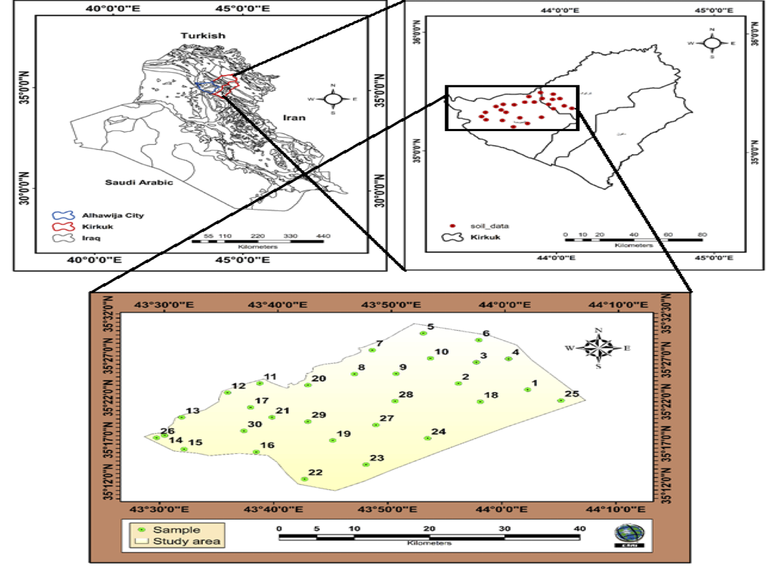
Map of soil samples in the study area.
Soil sampling and laboratory procedures
The study was conducted in the Hawija region of Western Kirkuk Governorate, Iraq. The study area was selected based on satellite images, soil/vegetation maps, spatial information, and a field visit. According to reference information derived from maps, field surveys, and GPS, the coordinates of the region are between 43°30’0” and 44°10’0″ E, and 35°32’0″ and 35°12’0″ N—a total area of approximately 1080.59 km2 (Figure 1). The study region is characterized by an arid and semiarid climate with low rainfall and an increase of temperature in the summer season. The topography is level to gently sloping, and predominantly flat with low elevations. Rainfall primarily occurs during winter, with the rainy season ranging from November to April. According to the Köppen classification system, the region has a semiarid climate (Bsh); it receives an average annual rainfall of 150-250 mm. Summer temperatures range between 17°C and 28°C, with maximum temperatures exceeding 45°C and heat intensity levels surpassing 45°C as well. The soil composition of the Hawija region is primarily composed of river sediments, with summer temperatures exceeding 45 °C. These include aridisols and entisols, according to the soil classification of the study area (pedon description), with relatively low moisture content and geospatial variations in soil properties, particularly in calcium carbonate (CaCO3) and organic matter content. The major land use in the region is wheat, barley, corn, vegetables, fruit, and other crops. The irrigation method used is either surface irrigation (Zab River) or waterlogged irrigation.
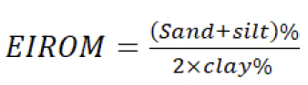
Soil quality index (SQI)
Calculated of soil quality indices using geometric method.
The assessment of soil quality was based on physical properties such as soil texture, bulk density, and erosion index (EIROM). Soil chemical properties included: EC, organic matter content, cation exchange capacity(CEC), CaSO4.2H2O and calcium carbonate (CaCO3), total nitrogen (NT %), and available phosphorus (Pavailable). These soil criteria and their degradation factors were classified based on resources (FAO, 2006; ; ; ; (Table 1).
Geometric Soil Quality Index (GSQI) = (Texture × Eirom × BD× CaCO3 × EC ×pH CaSO4.2H2O × CEC × OM × Total N×P_available ) ^1/n
Table 1 represents a quantitative assessment system for soil characteristic indices. The weighted grade was employed to convert physical and chemical measurements into numerical values that ranged from one (good quality) to two (very poor quality) and then be integrated into a single comprehensive indicator. This approach is based on the principle of a standard equation utilized in the evaluation of soil quality and its degradation . Geometric soil quality index is classified: < 1.13 good, 1.13-1.45 moderate, >1.45 poor, according to Kosmas et al., (1999).
Soil quality index calculating using fuzzy logic.
Soil Quality Index Calculation using Fuzzy logic. The standardized scores were integrated using a weighted additive method, a transparent and widely used approach for constructing soil quality indices ; ; ; . Because the weights sum to one and the membership scores range from 0 to 1, FSQI also ranges from 0 to 1. For presentation on a 0–100 scale. A larger FSQI indicates that the combined soil indicators are closer to the adopted desirable region conditions. The weighted additive model is compensatory; consequently, a high score for one indicator may partly offset a severe limitation in another. The ranges mentioned in Table 1 were used to determine the soil quality index using the Fuzzy method.
Fuzzy membership functions
Fuzzy logic was applied to convert measured soil characteristics into normalized membership values ranging from 0 to 1. Values close to one show optimal/good soil conditions, whereas values close to zero indicate soil properties with severe limitations. Where Lj is the lower critical value, and Uj is the upper reference value. When more than two scientifically meaningful control points were presented, linear interpolation was applied between successive points (xm, sm) and (xm + 1, sm + 1).
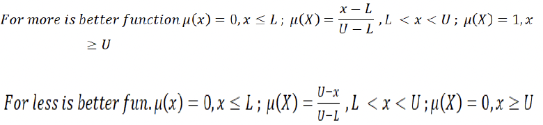
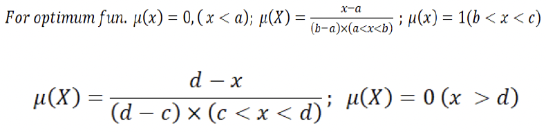
Where aj and dj are the lower and upper unacceptable limits, respectively, and bj and cj define the optimum interval. This function preserves a full membership score across the optimum pH range while allowing gradual decline toward the acidic and alkaline extremes.
Table 1: The soil physical and chemical analysis to calculate of soil quality index.
| Soil properties | Class | Description | Range | Score |
| Soil texture | 1 | Extreme | Clay loam | 1 |
| 2 | Very good | Silty clay loam, loam, silty clay, silt | 1.2 | |
| 3 | Good | Silt loam, clay < 60% | 1.4 | |
| 4 | Moderate | Sandy clay, sandy clay loam, sandy loam | 1.6 | |
| 5 | Low | Clay > 60% | 1.8 | |
| 6 | Very low | Loamy sand, Sand | 2 | |
BD-Bulk density Mg m-3 | 1 | Very high quality | ≤1.2 | 1 |
| 2 | High quality | 1.2-1.4 | 1.4 | |
| 3 | Moderate quality | 1.4-1.6 | 1.6 | |
| 4 | Low quality | 1.6-1.8 | 1.8 | |
| 5 | Very low quality | ≥ 1.8 | 2 | |
| EIrom | 1 | Very high quality | 1.5 | 1.0 |
| 2 | High | 1.5-4.0 | 1.2 | |
| 3 | Moderate | 4.0-8.0 | 1.5 | |
| 4 | Low | 8.0-12.0 | 1.8 | |
| 5 | Very low quality | >12 | 2 | |
| EC dSm-1 | 1 | Very high quality | 0-2 | 1 |
| 2 | High | 2.1-4 | 1.2 | |
| 3 | Moderate | 4.1-8 | 1.5 | |
| 4 | Low | 8.1-16 | 1.8 | |
| 5 | Very low quality | ≥16 | 2 | |
| pH | 1 | Neutral | 6.6-7.3 | 11.2 |
| 2 | Slightly alkaline | 7.3-7.9 | 1.5 | |
| 3 | Moderately | 7.9-8.4 | 1.8 | |
| 4 | Stronge | 8.4-9.0 | 2.0 | |
| CaCO3% | 1 | Very low quality | >40% | 2 |
| 2 | Low | 40-15 | 1.8 | |
| 3 | Moderate | 15-5 | 1.5 | |
| 4 | High | 5-2 | 1.2 | |
| 5 | Very high quality | <2% | 1 | |
| CaSO4 2H2O % | 1 | Very low quality | >40 | 2 |
| Low | 40-25 | 1.8 | ||
| 2 | Moderate | 25-5 | 1.5 | |
| 3 | High | 5-2 | 1.2 | |
| 4 | Very high quality | <2 | 1 | |
| OM % | 1 | Very high quality | >3 | 1 |
| 2 | High | 3 -2 | 1.2 | |
| 3 | Moderate | 2-1 | 1.5 | |
| 4 | Low | 1-0.5 | 1.7 | |
| 5 | Very low quality | ≤0.5 | 2 | |
| CEC Cmolkg-1 | 1 | Very low quality | <4 | 2 |
| 2 | Low | 4-10 | 1.8 | |
| 3 | Moderate | 10-20 | 1.5 | |
| 4 | High | 20-40 | 1.2 | |
| 5 | Very high quality | 40< | 1 | |
Ntotal % | Low | <0.1 | 2 | |
| Medium | 0.1-0.2 | 1.5 | ||
| High | 0.2< | 1 | ||
Pavialable mg kg-1 | Low | 5> | 2 | |
| Medium | 5-10 | 1.7 | ||
| High | 10-15 | 1.3 | ||
| Very high | >15 | 1 |
Entropy weight
Objective weights were calculated using the entropy weight method to reduce subjectivity in indicator weighting.

Table 2: The score of FSQI and quality classes.
| FSQI range (0–1) | Equivalent range (0–100) | Final evaluation |
| 0.00 ≤ FSQI < 0.20 | 0 ≤ FSQI < 20 | Very Poor |
| 0.20 ≤ FSQI < 0.40 | 20 ≤ FSQI < 40 | Poor |
| 0.40 ≤ FSQI < 0.60 | 40 ≤ FSQI < 60 | Moderate |
| 0.60 ≤ FSQI < 0.80 | 60 ≤ FSQI < 80 | Good |
| 0.80 ≤ FSQI ≤ 1.00 | 80 ≤ FSQI ≤ 100 | Very Good |
ArcGIS Software & Techiques interpolation
Inverse distance weighting (IDW)
Spatial interpolation techniques are commonly used to analyze or assess missing values using known values at study sites. The fundamental principle is that samples closer to the prediction location have a greater influence on the measured value than samples farther away or in other directions. The two most powerful factors in the method are: the number of adjacent soil points used in the approximation (based on any property, such as nitrogen, used in the approximation, which affects the smoothness of the area, and the control factor, which controls how quickly the weight decreases with increasing distance (range) . The Excel software was used to calculate descriptive statistics and plot curves of soil indices. Inverse Distance Weighting (IDW) is a deterministic spatial interpolation technique used to estimate values at unsampled sites from a set of known observations distributed across a geographical region. The method is based on the principle that the contribution of each sampled point to the predicted value decreases with increasing distance from the prediction sites. Consequently, nearby observations exert a stronger effect on the assessed value than observations sited farther away .
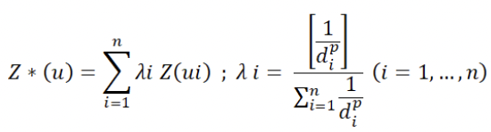
Where Z*(u) = represents the interpolated value at the unsampled area u; Z (ui) =denotes the observed value at sampling site ui; di = represents the distance between the prediction site and the ith sampled point. λi =denotes the weight assigned to the ith sampled observation and is calculated using the equation.; p =is the power parameter that controls the impact of distance on the weighting process.
Kriging models tests
GS+ (Geostatistics for the Environmental Sciences, Version 10), developed by Gamma Design Software, LLC, was used for geostatistical analyses. The software was employed to quantify and characterize the spatial relationships among soil characteristics. It is capable of handling different data distributions and spatial trends, is relatively robust to outliers, and can accommodate datasets with changing sampling densities. In addition, GS+ enables prediction of soil property values in unsampled areas based on observed values. The software was used to perform semivariogram and cross-semivariogram analyses to characterize spatial variability and to calculate the input parameters required for the kriging model. Moreover, this software demonstrated high efficiency in identifying the optimal model, such as a linear model, and achieving the highest coefficient of determination (R²), providing a more straightforward and specialized workflow than the ArcGIS program. (linear Model, spherical, gaussian, and exponential). The autocorrelation function and correlogram were calculated according to the following equation (Nielson and Wendroth, 2003; :

Where σ2:Variance. Z: Spatial values of the variable.;Xi: Station number; N: Number of spatial stations; Ż: Mean value of the variable; h: The separation distance between two stations.
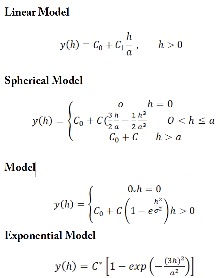
Where: Nugget (C₀) = local variation; Sill (C₀ + C₁) = statistical variance; Partial sill (C₁) = spatially structured component; Range (a)= effective distance of spatial effect.
Spatiality dependent = nugget/(nugget + sill) × 100
The spatial dependence classes: Strong <25%; Moderate 25–75%; Weak >75% .
Results and Discussion
Descriptive statistical of soil indices
The results of Table 2 showed variance in important soil properties such as soil texture. The sand percent (sand %) ranged between 20.0 and 88.0%, with an average of 51.4%; silt ranged between 4.0 and 70.0%, with an average of 41.3%; and clay ranged from 2.0 to 12.0%, with a mean of 7.4%. These ranges of different compositions, with moderate standard deviation SD, refer to distinguished heterogeneity in sediment sources and soil formation processes, which is consistent with alluvial surroundings in arid and semiarid regions. While the CV coefficients reach 32.1%, 41.7%, and 38.2% for sand, silt, and clay, respectively, confirming moderate to high spatial variability, a pattern usually detected in soils influenced by varying moisture regimes. The positive values of the skewness factor in sand and clay percent suggest that higher values dominate in certain microsites. In contrast, the negative skewness in silt implies fewer high-silt-percent observations. Such variances in soil texture strongly regulate soil hydraulic performance, soil aeration, and fertility element holding . Bulk density (BD) ranged between 1.2 and 1.5 Mg m-³, with a mean of 1.4 Mg m-³, a low standard deviation (0.1), and a CV of 4.9%, reflecting a generally typical distribution in the region. Higher values of bulk density typically reduce penetration and explain the effect on soil quality . The results showed that electrical conductivity ranged between 0.1 and 8.3 dS m-1, with a very high CV that reached143.5%. The pronounced positive skewness (3.2) indicates that soils are low in salinity in most samples. In contrast, samples with high salinity occur irregularly—likely representative of covers influenced by dismanagement . Organic matter (OM) content was usually low, ranging from 0.3 to 3.8%, with a mean of 1.4%, reflecting reduced biomass and rapid mineralization under arid conditions. A relatively high increase of CV (51.0%) reveals that extensive variability may be linked to variations in vegetation density and land cover/land use forms. The positive skewness (1.6) suggests that OM enrichment is uncommon and restricted to localized microsites. The negative correlation between OM and BD is due to the role of soil organic matter in soil stability, aggregate formation, and reduced soil compaction . Calcium carbonate (CaCO₃) content ranged from 27.7 to 39.8% with a mean of 33.2%, a low SD (3.2), and a CV (9.8%), which are characteristic of calcareous soils formed under arid conditions. The high values of calcium carbonate reflect soil alkalinity, slow movement of soluble micronutrients, and limit the availability of phosphorus through the Ca-P phase (FAO, 2022). Gypsum contents range from 0 to 10.5%, with a high CV value of 297.8% and very high positive skewness (3.8). Total nitrogen (TN) ranges from 0.1 to 0.3%, with an average of 0.1%, as expected due to decreases in soil organic matter, coarse soil texture, and other factors. The CV (41%) may reflect variability in plant distribution, plant residue patterns, and fertilization. Positive skewness (1.5) again indicates that most sites have minimal total nitrogen, with only limited enrichment zones. Available phosphorus (P) ranged from 3.5 to 29.8 mg kg-1 (mean = 9.7 mg kg-1), with a coefficient of variation of 54.7%, indicating substantial variability in phosphorus dynamics in the study area. In calcareous soils, the availability of phosphorus is strongly influenced by Ca-P compounds, which explains the commonly observed decrease in concentration. The positive skewness (2.5) suggests the presence of a limited phosphorus-rich region, likely linked to fertilizer residues or increased organic matter content . Collectively, the statistical indicators reveal that soil quality indicators controlled primarily by inherent pedogenic processes (e.g., calcium carbonate) tend to exhibit little variability. In contrast, attributes influenced by hydrological properties, land use, microtopography, and vegetation density (e.g., organic matter, phosphorus, and soil gypsum content) show high geospatial heterogeneity (Table 3).
Soil pedological indices
The results of Figure 2 and Figure 3 show the distribution of soil physical and chemical properties in the region, with quality ranging from very high to very low. The soil texture group ranges from a moderate soil quality class with an area of 761.27 km² and a percentage of 70.43%, to a high class of soil quality (H) with a percentage of area reaching 23.25% of the study area. This variance pattern indicates that the study area is dominated by medium texture, which is considered promising for agriculture, as it provides an equilibrium among various soil features. The bulk density values are classified into two classes: the moderate class reaches 60.59%, while the high-quality class reaches 39.41%, representative of a moderate grade of soil compaction, low permeability, and movement of water /aeration . The electrical conductivity ranged between the high-quality class, with an area of 89.44%, and the very high-quality class, with an area less than high. The results revealed that electrical conductivity values fell within the high and very high quality classes, with a value of 89.44%. This decreased electrical conductivity (high quality) is a good indicator of soil salinity because high electrical conductivity may reflect the accumulation of dissolved salts, such as sodium or chloride, in the surface layer, which affects crop growth (FAO, 2002). High salinity levels reduce the availability of nutrients such as iron and phosphorus . The results of the survey indicate the dominance of the high-quality gypsum-content variety, covering an area of 1000.18 km² with a percentage of 92.56%. This is followed by the high-quality class (H), covering an area of 65.99 km² and accounting of 11.6%. This confirms that the study area does not suffer from the problem of high gypsum levels, which is a determining indicator of agricultural production and affects the availability of many nutrients in the soil through the interaction of calcium ions with other ions important for plants, such as phosphorus. Gypsum affects soil permeability, aggregate stability, erosion activity, and water and air movement . The cation exchange capacity (CEC) was moderate (M), with an area of 1070.83 km² and a percentage of 99.10%. This perhaps provides an important note on sustainable soil addition of soil fertility enhancers. Therefore, cation exchange capacity plays an important role in supplying plants with nutrients, as its primary sources are either organic matter or high clay content . The total nitrogen content ranged from a low level (1.21%) to a moderate level (a very large area of 94.62%) and a high level (4.17%) in the study area. Therefore, there is a correlation among nitrogen content, cation exchange capacity, and low gypsum content. The moderate class (M) represented 94.62% of the total area. The total nitrogen content ranged from a low level (1.21%) to a moderate level (94.62%) and a high level (4.17%) in the study area. Therefore, there is a correlation between nitrogen content, cation exchange capacity, and low gypsum content . Phosphorus in the soil is considered a key element for life. Phosphorus content was classified into four main categories: low-quality soil, covering 13.52 km²; medium-quality soil, covering 682.77 km² (63.18%) of the study area, the largest area; high-quality soil, covering 326.88 km² (30.25%); and a specific area with very high phosphorus content, representing 5.31%. This significant variation is likely due to differences in sustainable management practices between different sites. Therefore, phosphorus is considered one of the essential elements that plays a significant role in agricultural production and soil fertility. The relatively low organic matter observed in the study region may reflect limited carbon inputs and continuous soil disturbance, as long-term field observations show that residue retention and reduced tillage increase soil organic carbon and improve several soil-health functions compared with conventional management . The limitation of available phosphorus is particularly consistent with the calcareous nature of the soils. Despite these fertility constraints, the overall soil-quality class remained relatively favorable because the SQI represents the integrated contribution of several indicators rather than any single property . In the present study, the favorable status of EC and CaSO₄ therefore reduced the overall chemical limitation. In contrast, organic matter and available P acted as comparatively weaker components of the integrated index. Low salinity is particularly important because increasing EC restricts plant growth, while moderate or low gypsum contents generally impose limited adverse effects on crop performance. Finally, the spatial differences among sampling locations are consistent with recent geostatistical studies showing substantial spatial variability in SOC, EC, and available P, and supporting site-specific rather than uniform soil management; however, because management history was not directly measured here, these factors should be regarded as plausible rather than confirmed drivers .
Table 3: Statistical descriptive of soil pedological characterize
| Statistical criteria | Soil texture % | Bulk dinsity | EIROM | EC | CEC | OM | CaC O3 | CaSO4.2 H2O | TN | P | ||
| Sand | Silt | Clay | Mgm-3 | dSm-1 | CmolKg-1 | % | % | mg kg-1 | ||||
| Minimum | 20.0 | 4.0 | 2.0 | 1.2 | 3.7 | 0.1 | 13.8 | 0.3 | 27.7 | 0.0 | 0.1 | 3.5 |
| Maximum | 88.0 | 70.0 | 12.0 | 1.5 | 24.5 | 8.3 | 21.5 | 3.8 | 39.8 | 10.5 | 0.3 | 29.8 |
| Average | 51.4 | 41.3 | 7.4 | 1.4 | 7.7 | 1.2 | 16.8 | 1.4 | 33.2 | 0.8 | 0.1 | 9.7 |
| S.D. | 16.5 | 17.2 | 2.8 | 0.1 | 4.4 | 1.7 | 2.2 | 0.7 | 3.2 | 2.3 | 0.1 | 5.3 |
| CV % | 32.1 | 41.7 | 38.2 | 4.9 | 57.8 | 143.5 | 13.2 | 51.0 | 9.8 | 297.8 | 41.0 | 54.7 |
| Skew | 0.3 | -0.3 | 0.1 | -0.5 | 2.5 | 3.2 | 0.3 | 1.6 | 0.3 | 3.8 | 1.5 | 2.5 |
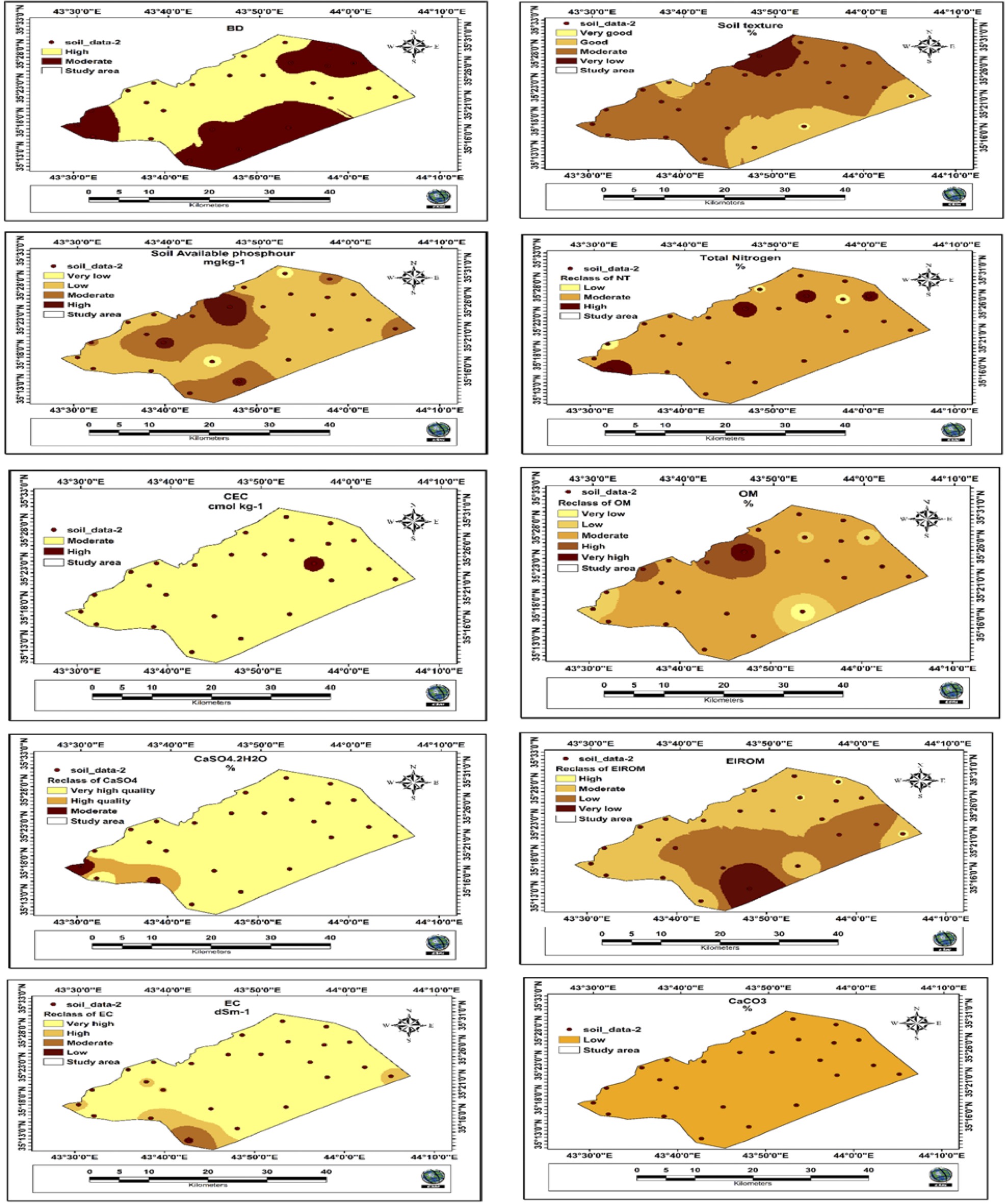
Mapping spatial distribution of soil quality criteria.
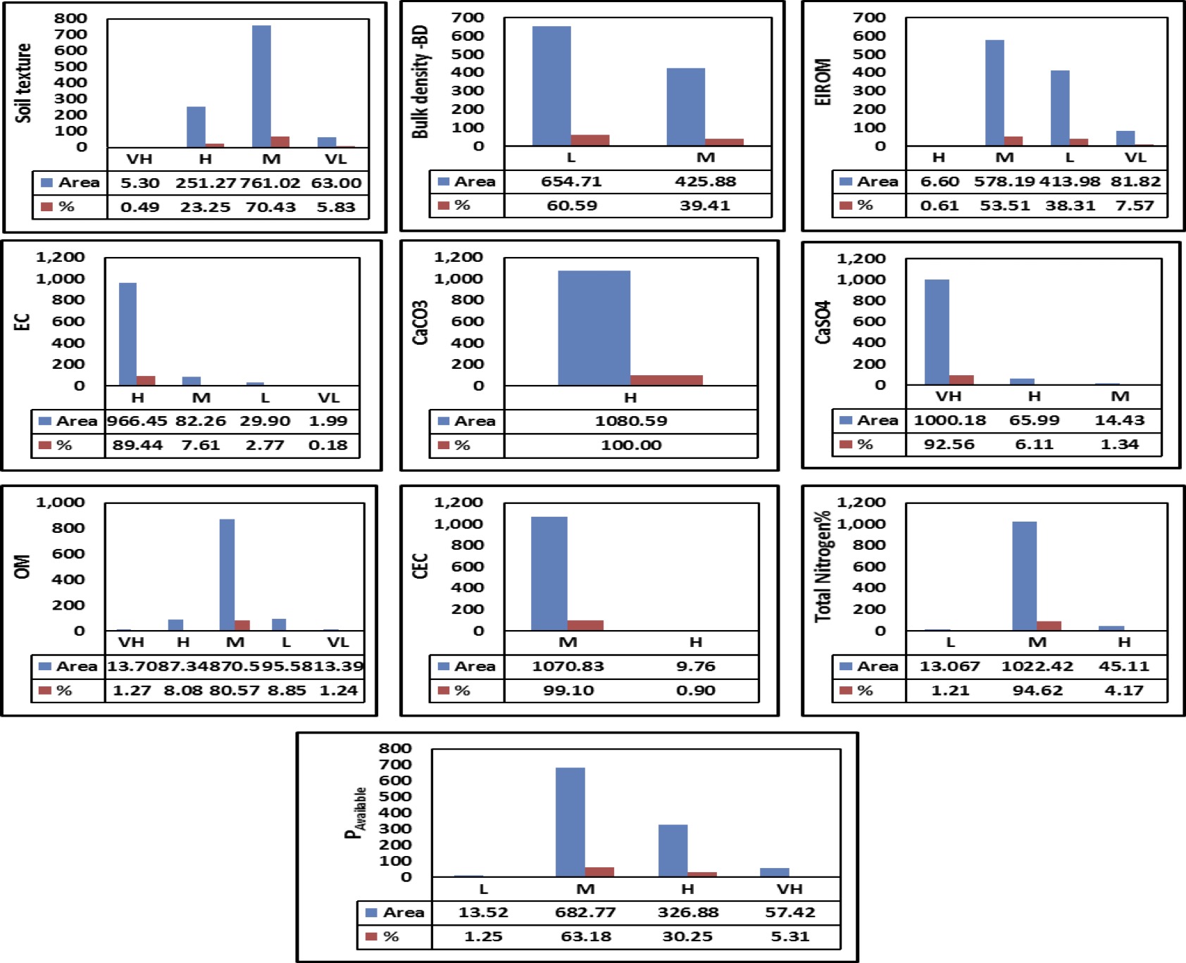
Spatial distribution classes of soil quality indices in the study area
Kreging interpolation& semivariogram interpretation
The semivariogram analysis revealed a distinct spatial variation for most of the studied soil properties (Figure 4; Table 4) and according to the classification proposed by Cambardella et al. (1994), soil reaction, calcium carbonate, gypsum, organic matter, cation exchangeable capacity, total nitrogen, bulk density, and erosion index (EIrom) exhibited strong spatial dependence (SP), whereas phosphorus availability showed moderate dependence. Strong spatial dependence indicates that a substantial part of the observed variability is spatially structured at the sampling scale rather than dominated by unresolved local variation. Similar spatial organization of soil physicochemical properties has been reported in recent geostatistical studies by Abdu et al. (2023) and Wani et al. (2024). Among the investigated properties, pH and BD showed the most robust spatial structures, combining strong spatial dependence with the highest semivariogram fits (R2 = 0.86 and 0.88, respectively). These differences indicate that the strength of spatial dependence should not be considered synonymous with the quality of semivariogram fitting or prediction accuracy. The importance of combining variogram modelling with prediction assessment has also been emphasized in recent soil-mapping studies. The spatial ranges also differed considerably among soil characteristics, indicating that they operate at different scales. Available P, OC, and BD showed relatively long spatial ranges, suggesting broader-scale continuity across the study site. In contrast, TN displayed a shorter range and therefore greater variation over shorter distances. The exceptionally large range obtained for EIrom, together with its low R2, warrants particular caution. Such a result should be evaluated against the dimensions of the study area and the maximum sampling distance before being interpreted as a physically meaningful correlation distance. Available P was the only confirmed property showing moderate spatial dependence, indicating a greater contribution of local-scale variability than observed for the strongly structured properties. This pattern may reflect the sensitivity of available P to spatially heterogeneous soil conditions and management practices. Comparable spatial variabilityof soil nutrient availability has been reported in field-scale geostatistical investigations. Overall, the results demonstrate substantial spatial organization of most soil properties, supporting their suitability for geostatistical mapping.
Geometric and fuzzy logic methods
The results of Figure 5 and Figure 6 show that the pointer used to estimate of soil system by using various chemical, fertilizer and physical factors into a only assessable value. These indices are reflect a vital diagnostic device in modern pedological science for assessing the productive capability and agricultural lands sustainability . GSQI varied from 1.047 to 1.239, with a mean of 1.1267 and a median of 1.118. The mean was only 0.0033 index units below the Good-Moderate threshold of 1.13, and 13 of the 25 sites (52%) lay within ±0.03 of that boundary (Table 5). This confirms that much of the sample was concentrated near the principal decision threshold, so modest changes in the underlying indicators can alter class assignment without implying a large change in overall soil condition. Sixteen sites (64%) were Good, and nine (36%) were Moderate. The interquartile range was 0.044, and the coefficient of variation was 4.08%. Because GSQI is bounded and has no meaningful zero, CV is retained only as
Table 4: Kreging interpolation model of soil properties using GS+ program.
| Kriging Models | Nugget(C0) | Sill(C0+C) | Range (m) | model | R2 | Spatiality dep. | Classes of S.d |
| pH | 0.00 | 0.07 | 12159 | Gaussian | 0.86 | 0.14 | S |
| EC | 0.01 | 0.05 | 2.93 | Linear | 0.77 | 20 | W |
| CaCO3 | 0.01 | 8.44 | 9249.15 | Gaussian | 0.77 | 0.12 | S |
| CaSO4 | 0.01 | 3.73 | 8140.64 | Gaussian | 0.34 | 0.27 | S |
| OC | 0.02 | 0.27 | 17459.07 | Gaussian | 0.76 | 7.41 | S |
| NT | 0 | 0 | 6130 | Spherical | 0.21 | 0.28 | S |
| P | 20.99 | 41.99 | 19433.61 | Gaussian | 0.25 | 49.99 | M |
| BD | 0 | 0.01 | 17511.03 | Gaussian | 0.88 | 0 | S |
| CEC | 0.01 | 4.73 | 9075.95 | Gaussian | 0.65 | 0.21 | S |
| EIrom | 12.9 | 52.64 | 183300 | exponential | 0.17 | 24.51 | S |
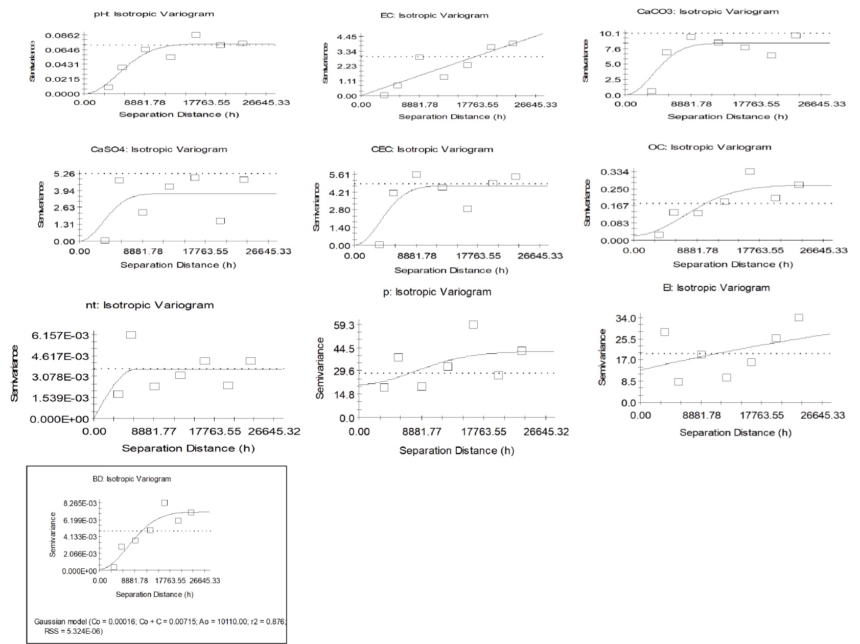
The autocorrelation analysis diagrams of soil properties using kriging model.
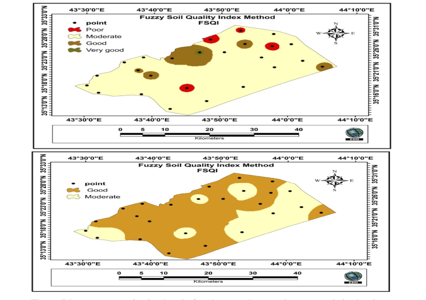
Spatial distribution of soil-quality classes using the two index frameworks.
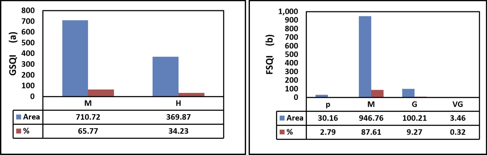
Areal distribution of soil quality classes: (a) GSQI and (b) FSQI.
a within-index descriptor. The restricted spread is consistent with the bounded 1-2 scoring domain and geometric aggregation of the indicator scores. FSQI covered a substantially broader numerical interval within its own scale, from 30.964 to 84.528, with a mean of 51.543 and a median of 49.470. Site classification produced four levels: 4 sites (16%) were Poor, 14 (56%) were Moderate, 6 (24%) were Good, and 1 (4%) was Very Good. The distribution showed only mild positive skewness (0.505), and the coefficient of variation was 24.34%. The wider separation of FSQI scores and the presence of four site-level classes indicate greater differentiation of the sampled locations within this fuzzy scale. That pattern is compatible with continuous membership functions, which preserve intermediate degrees of performance instead of converting every indicator directly at a hard boundary . Nevertheless, the observed differentiation also depends on the selected membership functions, weights, and class limits; it should therefore be described as greater discrimination in this dataset rather than as evidence of intrinsically greater accuracy ; .
Table 5: Statistical summary of GSQI and FSQI for soil sampling sites.
| Statistical parameter | GSQI | FSQI |
| Mean | 1.1267 | 51.543 |
| Standard deviation (SD) | 0.0460 | 12.545 |
| Standard error (SE) | 0.0092 | 2.509 |
| 95% CI of the mean | 1.1077-1.1457 | 46.365-56.721 |
| Median | 1.118 | 49.470 |
| First quartile (Q1) | 1.100 | 42.814 |
| Third quartile (Q3) | 1.144 | 60.316 |
| Interquartile range (IQR) | 0.044 | 17.502 |
| Minimum | 1.047 | 30.964 |
| Maximum | 1.239 | 84.528 |
| Range | 0.192 | 53.564 |
| Coefficient of variation (%) | 4.08 | 24.34 |
| Skewness | 0.831 | 0.505 |
| Excess kurtosis | 0.946 | 0.535 |
| Shapiro-Wilk W | 0.943 | 0.966 |
| Shapiro-Wilk P-value | 0.178 | 0.549 |
| Direction-aligned Spearman correlation | rho = 0.167 | P = 0.424 |
Neither index showed a statistically significant departure from normality according to the Shapiro-Wilk test (GSQI: W = 0.943, P = 0.178; FSQI: W = 0.966, P = 0.549). Normality, however, does not make the two raw means directly comparable because their scales and directions of measurement differ. GSQI was therefore direction-aligned only for ranking purposes and Spearman’s correlation was used as the primary between-method test. The association was weak and non-significant (rho = 0.167, P = 0.424), indicating that the two formulations did not consistently preserve site ordering. Because both indices were derived from the same soil dataset, this weak correspondence is most reasonably attributed to differences in scoring and aggregation structure rather than to a simple shift in numerical scale ; . The GSQI map assigned 710.72 km² (65.77%) of the 1080.59 km² study area to the Moderate class and 369.87 km² (34.23%) to the Good class. This spatial pattern differs markedly from the site-frequency result, in which Good sites accounted for 64% of observations. The result is especially plausible given that the GSQI sample mean lies very close to the 1.13 Good-Moderate boundary, so modest spatial changes around that threshold can alter the extent of the reclassified raster without implying an error in the site calculations. FSQI produced a stronger concentration in the intermediate class. Moderate soil quality occupied 946.76 km² (87.61%), compared with 100.21 km² (9.27%) of Good, 30.16 km² (2.79%) of Poor, and 3.46 km² (0.32%) of Very Good land. Moderate represented 56% of sampling sites but 87.61% of the mapped area, whereas Poor sites accounted for 16% of observations but only 2.79% of the area. The dominance of broad intermediate zones most likely reflects the combined influence of continuous fuzzy scoring, the spatial configuration of the sampled values, IDW interpolation, and the adopted class thresholds. Accordingly, the mapped proportions should be interpreted as model-based spatial estimates rather than as direct extensions of site frequencies.
IDW estimates values at unsampled locations from neighboring measurements; consequently, class area depends on sample configuration, local gradients, interpolation settings, and reclassification thresholds ; . FSQI assigned 236.04 km² more land to the Moderate class than GSQI, a difference of 21.84 percentage points. Conversely, descriptively grouping FSQI Good and Very Good gives 103.67 km² (9.59%) of favorable land, compared with 369.87 km² (34.23%) under GSQI. These marginal totals reflect method-dependent spatial classification, but spatial agreement should be quantified only from a cell-by-cell overlay of the original raster surfaces (Figure 2). They differ, however, in how sharply they partition the same underlying information. GSQI places a larger fraction of the landscape in the favorable category. In contrast, FSQI allocates most of the area to Moderatequality and retains small Poor and Very Good zones. This is a method effect rather than a contradiction. The geometric formulation summarizes a bounded set of indicator scores using a multiplicative composite, while fuzzy logic preserves continuous degrees of membership before final classification. Previous SQI comparisons likewise show that methodological choices can change the numerical response and class structure of an index ; ; . The weak rank correlations found here provide dataset-specific evidence that the two formulations should be interpreted as complementary representations ratherthan interchangeable measurements. For sustainable management, a Moderate composite class should be treated as a diagnostic signal rather than a fertilizer or amendment prescription. Soil-quality indices summarize multiple functions and constraints, and similar composite scores can arise from different combinations of limiting properties ; . For sustainable management, a Moderate composite class should be treated as a diagnostic signal rather than a fertilizer or amendment prescription. Soil-quality indices summarize multiple functions and constraints, and similar composite scores can arise from different combinations of limiting properties ; . Management decisions should therefore return to the underlying indicators measured at each location - for example, organic matter, nutrient availability, salinity, bulk density, or erosion status - before selecting an intervention. The small Poor area identified by FSQI is a logical priority for field verification and targeted rehabilitation. In contrast, favorable zones are better approached through maintenance and monitoring unless a specific indicator shows a constraint. This indicator-led use of spatial SQI information is consistent with digital soil mapping and management-zone approaches designed to support site-specific management and more efficient allocation of agricultural inputs ; ; .
Conclusions and Recommendations
The papers exposed the main geospatial variation in the pedological soil properties. Soil texture classes ranged from high quality to moderate quality, covering a large area of the study area. In contrast, soil bulk density and erosion index (EIROM) qualities ranged from moderate (M) to low (L) classes. On the other hand, soil organic matter %, total nitrogen %, and CEC (C mol kg-1) were mostly in the medium class. This will likely influence sustainable management of lands. The gypsum percent and electrical conductivity (dSm-1) ranged from high (H) to very high (VH) quality, posing a danger only to particular sites within the area. The spatial assessment of soil quality identified two quality classes only, Moderate and High, under both the FSQI and GSQI approaches; however, their spatial proportions differed markedly between the two methods. Under the FSQI, the high class (H) was dominant, accounting for ≈ 92.91%, while the moderate class (M) accounted for only 7.09%. In contrast, the GSQI indicated a broader distribution of the moderate class (M), which accounted for ≈ 65.77%, while the High class (H) accounted for 34.23%. These findings indicate that soil quality classification is determined not by a single soil property but by the combined effect of all selected indices. Therefore, the final class reflects the overall balance among soil fertility, organic matter status, and other functional soil attributes. From a sustainable land-management perspective, the predominance of the high class under FSQI suggests the presence of relatively favorable soil status. In contrast, the larger extent of the moderate class under GSQI indicates the existence of manageable constraints that still require attention. Accordingly, sustainable management should focus on maintaining and protecting High-quality areas from degradation. In contrast, Moderate areas should be prioritized for targeted interventions, particularly through soil fertility improvement, enhancement of organic matter, and conservation agriculture practices.
Acknowledgments
The authors’ thanks of Tikrit universty, agricultural college, and Soil sciences and Water Resources that provided assistance for research achaive and enable analysis of laboratory.
Novelty Statement
This study proposes a novel integrated methodology for soil quality evaluation by incorporating pedological soil quality indicators with comparative weighting strategies based on Weighted Average and Fuzzy Logic approaches. The combination of these methods with spatial prediction models (Inverse Distance Weighting and Kriging) enables a more reliable characterization and mapping of soil quality variability in arid and semi arid in Iraq.
Author’s Contribution
Saja Omer Hussien: Conducted the field investigations, georeferencing of sampling sites, and laboratory analyses.
Ayad Abdullah Khalaf: Performed data validation, statistical analyses, programming of soil quality index models, spatial interpolation using IDW and Kriging methods, and map generation.
Both authors contributed to data interpretation, manuscript writing, revision, and final approval of the manuscript.
Generative AI and AI-assisted technology statement
The authors declare that no generative AI and AI assisted technology was used in the creation of this manuscript.
Conflict of interest
The authors have declared no conflict of interest.
References
- Abdu, A., F. Laekemariam, G. Gidago, A. Kebede and L. Getaneh. 2023. Variability analysis of soil properties, mapping, and crop test responses in Southern Ethiopia. Heliyon., 9: e14013. https://doi.org/10.1016/j.heliyon.2023.e14013 [CrossRef]
- Abidin, A.R. and M. Mukri. 2002. Establishment of Soil Erosion Scale With Regards to Soil Grading Characteristic. In: 2nd World Engineering Congress. Sarawak, Malaysia., pp. 235-239.
- Abidin, R.Z., M.S. Sulaiman and N. Yusoff. 2017. Erosion risk assessment: A case study of the Langat River bank in Malaysia. Int. Soil Water Conservat. Res., 5: 26-35. https://doi.org/10.1016/j.iswcr.2017.01.002 [CrossRef]
- Andrews, S.S., D.L. Karlen, and J.P. Mitchell. 2002. A comparison of soil quality indexing methods for vegetable production systems in Northern California. Agriculture, Ecosys. Environ., 90(1): 25-45 https://doi.org/10.1016/S0167-8809(01)00174-8 [CrossRef]
- Arévalo-Hernández, J.J., E.M. de Oliveira, G.A.E.S Ferraz,. D.C. Polanía-Montiel, Liscano A.L. Solano, and M.L.N. Silva. 2024. The delineation of management zones using soil quality indices for the cultivation of irrigated rice (Oryza sativa L.) in Huila, Colombia. Geoderma Region., 39: e00886. https://doi.org/10.1016/j.geodrs.2024.e00886 [CrossRef]
- Askari, M.S., S.M. O’Rourke and N.M. Holden. 2015. Evaluation of soil quality using VNIR spectroscopy. Geoderma., 243: 80-91. https://doi.org/10.1016/j.geoderma.2014.12.012 [CrossRef]
- Baveye, P.C., J. Baveye and J. Gowdy. 2016. Soil ecosystem services and natural capital. Front. Environ. Sci., 4: 41. https://doi.org/10.3389/fenvs.2016.00041 [CrossRef]
- Bel-Lahbib, S., K. Ibno Namr, B. Rerhou, F. Mosseddaq, B. El Bourhrami, and L. Moughli. 2023. Assessment of soil quality by modeling soil quality index and mapping soil parameters using IDW interpolation in Moroccan semi-arid. Model. Earth Sys. Environ., 9: 4135-4153 https://doi.org/10.1007/s40808-023-01718-1. [CrossRef]
- Biswas, S., P. Singh, R. Rahaman, K.V. Patil and N. De. 2023. Soil quality and crop productivity under 34 years old long-term rainfed rice based cropping system in an inceptisol of sub-tropical India. Front. Soil Sci., 3. https://doi.org/10.3389/fsoil.2023.1155712 [CrossRef]
- Blake, G.R. and K.H. Hartge. 1986. Bulk density. In: A. Klute (Ed.), Methods of Soil Analysis. Part 1. Physical and Mineralogical Methods, 2nd ed. American Society of Agronomy and Soil Science Society of America, Madison, WI. pp.363-375. https://doi.org/10.2136/sssabookser5.1.2ed.c13 [CrossRef]
- Bonilla-Bedoya, S., K. Valencia, M.Á. Herrera, M. López-Ulloa, D.A. Donoso and J.E. Macedo Pezzopane. 2023. Mapping 50 years of contribution to the development of soil quality biological indicators. Ecol. Indicat., 148. https://doi.org/10.1016/j.ecolind.2023.110091 [CrossRef]
- Bünemann, E.K., G. Bongiorno, Z. Bai, R.E. Creamer, G. De Deyn, R. de Goede, L. Fleskens, V. Geissen, T.W. Kuyper, P. Mäder, M. Pulleman, W. Sukkel, J.W. van Groenigen, and L. Brussaard. 2018. Soil quality - A critical review. Soil Biology and Biochemistry, 120, 105-125. https://doi.org/10.1016/j.soilbio.2018.01.030 [CrossRef]
- Cambardella, C.A., T.B. Moorman, J.M. Novak, T.B. Parkin, D.L. Karlen, R.F. Turco and A.E. Konopka. 1994. Field-scale variability of soil properties in central Iowa soils. Soil Sci. Soc. Amer. J., 58: 1501-1511. https://doi.org/10.2136/sssaj1994.03615995005800050033x [CrossRef]
- Chaudhry, H., H.B. Vasava, S. Chen, D.D. Saurette, A. Beri, A.W. Gillespie, and A. Biswas. 2024. Evaluating the Soil Quality Index Using Three Methods to Assess Soil Fertility. Sen., 24(3): 864. https://doi.org/10.3390/s24030864 [CrossRef]
- Cohen, J. 1960. A coefficient of agreement for nominal scales. Educat. Psychol. Measur., 20: 37-46. https://doi.org/10.1177/001316446002000104 [CrossRef]
- Doran, J.W. and T.B. Parkin. 1994. Defining and assessing soil quality. In: J.W. Doran, D.C. Coleman, D.F. Bezdicek and B.A. Stewart (Eds.), Defining Soil Quality for a Sustainable Environment. Soil Science Society of America, Madison, WI. pp.3-21. https://doi.org/10.2136/sssaspecpub35.c1 [CrossRef]
- Doran, J.W., M. Sarrantonio and M.A. Liebig. 1996. Soil health and sustainability. Adv. Agron., 56: 1-54. https://doi.org/10.1016/S0065-2113(08)60178-9 [CrossRef]
- El Behairy, R.A., H.M. El Arwash, A.A. El Baroudy, M.M. Ibrahim, E.S. Mohamed and D.E. Kucher. 2024. How can soil quality be accurately and quickly studied? A review. Agron. 14: 1682. https://doi.org/10.3390/agronomy14081682 [CrossRef]
- Fageria, N.K. and V.C. Baligar. 2005. Enhancing nitrogen use efficiency. Advan. Agron. 88: 97-185. https://doi.org/10.1016/S0065-2113(05)88004-6 [CrossRef]
- Fagerland, M.W., S. Lydersen and P. Laake. 2013. The McNemar test for binary matched-pairs data: Mid-p and asymptotic are better than exact conditional. BMC Medical Res. Methodol., 13: 91. https://doi.org/10.1186/1471-2288-13-91 [CrossRef]
- FAO. 2002. Agricultural Drainage Water Management in Arid and Semi-Arid Areas. FAO Irrigation and Drainage Paper 61. Rome: Food and Agriculture Organization of the United Nations. https://www.fao.org/docrep/005/y4263e/y4263e00.htm
- FAO. 2006. Guidelines for Soil Description, 4th ed. Food and Agriculture Organization of the United Nations, Rome.
- FAO. 2022. Handbook for Saline and Sodic Soils: Diagnosis and Reclamation. Food and Agriculture Organization of the United Nations, Rome.
- Gee, G.W. and J.W. Bauder. 1986. Particle-size analysis. In: A. Klute (Ed.), Methods of Soil Analysis. Part 1. Physical and Mineralogical Methods, 2nd ed. Americ. Soc. Agron. Soil Sci. Soc. America, Madison, WI. pp.383-411. https://doi.org/10.2136/sssabookser5.1.2ed.c15 [CrossRef]
- Ghosh, T., B. Das, D. Chakraborty, V.K. Singh, D. Das, P. Aggarwal, A. Sarkar, P.K. Jha and P.V.V. Prasad. 2025. Evaluation of soil quality frameworks in rice-wheat systems under integrated nutrient management in Indo-Gangetic Plains. Scienti. Repor., 15: 37511. https://doi.org/10.1038/s41598-025-21630-1 [CrossRef]
- Havlin, J.L., S.L. Tisdale, W.L. Nelson and J.D. Beaton. 2014. Soil fertility and fertilizers, 8th ed. Pearson.
- Hazelton, P. and B. Murphy. 2007. Interpreting Soil Test Results: What Do All the Numbers Mean? CSIRO Publishing. https://doi.org/10.1071/9780643094680 [CrossRef]
- Hillel, D. 2004. Introduction to Environmental Soil Physics. Elsevier/Academic Press, Amsterdam.
- Hyun, J.Y., J. Kim, A. Kim, A.F. Plante and G. Yoo. 2022. Ecosystem services-based soil quality index tailored to the metropolitan environment for soil assessment and management. Sci. Tot. Environ., 820: 153301. https://doi.org/10.1016/j.scitotenv.2022.153301 [CrossRef]
- Isaaks, E.H. and R.M. Srivastava. 1989. Applied Geostatistics. Oxford University Press, New York.
- Iticha, B., and C. Takele. 2019. Digital soil mapping for site-specific management of soils. Geoderma., 351: 85-91. https://doi.org/10.1016/j.geoderma.2019.05.026 [CrossRef]
- Jones, J.B., Jr. 2012. Plant nutrition and soil fertility manual, 2nd ed. CRC Press. https://doi.org/10.1201/b11577 [CrossRef]
- Kang, L., R. Zhao, K. Wu, Z. Feng, H. Zhao and S. Zhang. 2023. Distribution characteristics and influencing factors of soil biological indicators in typical farmland soils. Land 12:755. https://doi.org/10.3390/land12040755 [CrossRef]
- Karlen, D.L., M.J. Mausbach, J.W. Doran, R.G. Cline, R.F. Harris and G.E. Schuman. 1997. Soil quality: Concept, definition, and framework for evaluation. Soil Sci. Soc. Amer. J., 61: 4-10. https://doi.org/10.2136/sssaj1997.03615995006100010001x [CrossRef]
- Kaya, N.S. and O. Dengiz. 2024. Assessment of the neutrosophic Fuzzy-AHP and predictive power of some machine learning approaches for maize silage soil quality. Comput. Electron. Agric., 226: 109446. https://doi.org/10.1016/j.compag.2024.109446 [CrossRef]
- Khalaf, A.N. and M.A. Hussien. 2021. Environment Sensitivity Maps Of Land Degradation And Desrtification Using Medulas Model And Remote Sensing In Shirqat City/Iraq. https://doi.org/10.36103/ijas.v52i3.1361 [CrossRef]
- Kosmas, C., A. Ferrara, H. Briasouli, and A. Imeson. 1999. Methodology for mapping Environmentally Sensitive Areas (ESAs) to desertification. In C. Kosmas, M. Kirkby, and N. Geeson (Eds.), The MEDALUS Project: Mediterranean Desertification and Land Use. Manual on Key Indicators of Desertification and Mapping Environmentally Sensitive Areas to Desertification. European Union 18882, pp. 31-47.
- Kosmas, C., O. Kairis, C. Karavitis, C.J. Ritsema, L. Salvati, S. Acikalin, S. Alcala, P. Alfama, J. Atlhopheng, J. Barrera, A. Belgacem, A. Solé-Benet, J. Brito, M. Chaker, R. Chanda, C. Coelho, M. Darkoh, I. Diamantis, O. Ermolaeva, A. Ziogas. 2014. Evaluation and selection of indicators for land degradation and desertification monitoring: Methodological approach. Environ. Manag., 54: 951-970. https://doi.org/10.1007/s00267-013-0109-6 [CrossRef]
- Lal, R. 2015. Restoring soil quality to mitigate soil degradation. Sustainability 7:5875-5895. https://doi.org/10.3390/su7055875 [CrossRef]
- Lal, R. 2020. Soil organic matter and water retention. Agron. J., 112: 3265-3277. https://doi.org/10.1002/agj2.20282 [CrossRef]
- Li, K. and C. Wang. 2023. Multiple soil quality assessment methods for evaluating effects of organic fertilization in wheat-maize rotation system. Europ. J. Agron., 150: 126929. https://doi.org/10.1016/j.eja.2023.126929 [CrossRef]
- Minasny, B., A.B. McBratney and J. Padarian. 2022. Digital soil mapping: A review. Geoderma 409: 115-124.
- Mora-Herrera, D.Y., S. Guillaume, D. Snoeck and O. Zúñiga Escobar. 2020. A fuzzy logic based soil chemical quality index for cacao. Comput. Electron. Agric., 177: 105624. https://doi.org/10.1016/j.compag.2020.105624 [CrossRef]
- Mukherjee, A. and R. Lal. 2014. Comparison of Soil Quality Index Using Three Methods. PLOS ONE 9: e105981. https://doi.org/10.1371/journal.pone.0105981 [CrossRef]
- Nasir, M.J., M.F. Haider, Z. Ali, W. Akhtar and S. Alam. 2024. Evaluation of soil quality through Geometric soil quality index (SQI) of Tehsil Charsadda, Khyber Pakhtunkhwa, Pakistan. J. Saudi Soc. Agric. Sci., 23: 42-54. https://doi.org/10.1016/j.jssas.2023.09.001 [CrossRef]
- Nelson, D.W. and L.E. Sommers. 1996. Total carbon, organic carbon, and organic matter. In: D.L. Sparks (Ed.), Methods of Soil Analysis. Part 3. Chemical Methods. Soil Sci. Soc. America, Madison, WI. pp.961-1010. https://doi.org/10.2136/sssabookser5.3.c34 [CrossRef]
- Nielsen, D.R. and O. Wendroth. 2003. Spatial and Temporal Statistics: Sampling Field Soils and Their Vegetation. Catena Verlag, Reiskirchen, Germany, 398 p. Scientific Research Publishing [CrossRef]
- Nguemezi, C., P. Tematio, M. Yemefack, D. Tsozue and T. Silatsa. 2020. Soil quality and soil fertility status in major soil groups at the Tombel area, South-West Cameroon. Heliyon., 6: e03432. https://doi.org/10.1016/j.heliyon.2020.e03432 [CrossRef]
- Norris, C.E., G.M. Bean, S.B. Cappellazzi, M. Cope, K.L.H. Greub, D. Liptzin, E.L. Rieke, P.W. Tracy, C.L.S. Morgan and C.W. Honeycutt. 2020. Introducing the North American project to evaluate soil health measurements. Agron. J., 112: 3195-3215. https://doi.org/10.1002/agj2.20234 [CrossRef]
- Olsen, S.R. and L.E. Sommers. 1982. Phosphorus. In: A.L. Page (Ed.), Methods of Soil Analysis. Part 2. Chemical and Microbiological Properties. ASA-SSSA, Madison, WI. pp.403-430. https://doi.org/10.2134/agronmonogr9.2.2ed.c24 [CrossRef]
- Page, A.L., R.H. Miller and D.R. Keeney. 1982. Methods of Soil Analysis. Part 2. Chemical and Microbiological Properties, second edition. American Society of Agronomy. Inc. Soil Science Society of America, Inc, Number. 9 (part 2) in the series 1159.
- Parkin, T.B., J.W. Doran and E.J. Kladivko. 2022. Soil health: Assessing, measuring, and managing. J. Soil Water Conserv., 77: 332-348.
- Qi, Y., J.L. Darilek, B. Huang, Y. Zhao, W. Sun and Z. Gu. 2009. Evaluating soil quality indices in an agricultural region of Jiangsu Province, China. Geoderma. 149: 325-334. https://doi.org/10.1016/j.geoderma.2008.12.015 [CrossRef]
- Rodríguez, E., R. Peche, C. Garbisu, I. Gorostiza, L. Epelde, U. Artetxe, A. Irizar, M. Soto, J.M. Becerril and J. Etxebarria. 2016. Dynamic Quality Index for agricultural soils based on fuzzy logic. Ecol. Indicat., 60: 678-692. https://doi.org/10.1016/j.ecolind.2015.08.016 [CrossRef]
- Sarğın, B., P. Alaboz, S. Karaca and O. Dengiz. 2024. Pythagorean fuzzy SWARA weighting technique for soil quality modeling of cultivated land in semi-arid terrestrial ecosystems. Comput. Electron. Agric. 227: 109466. https://doi.org/10.1016/j.compag.2024.109466 [CrossRef]
- Shahid, S.A., M. Zaman and L. Heng. 2018. Introduction to soil salinity, sodicity and diagnostics techniques. In: Guideline for Salinity Assessment, Mitigation and Adaptation Using Nuclear and Related Techniques. Springer. https://doi.org/10.1007/978-3-319-96190-3_1 [CrossRef]
- Shepard, D. 1968. A two-dimensional interpolation function for irregularly spaced data. In: Proceedings of the 1968 ACM National Conference. ACM. pp.517-524. https://doi.org/10.1145/800186.810616 [CrossRef]
- Sparks, D.L. 2003. Environmental soil chemistry, 2nd ed. Academic Press/Elsevier. https://doi.org/10.1016/B978-012656446-4/50001-3 [CrossRef]
- Subhash, M., N.K. Sinha, J. Kumar, M. Mohanty, R.N. Sahoo, S. Jayaraman, N. Kumar, A. Rani, J.K. Thakur, A. Mandal, D. Kumar, R. Mishra and M. Prabhakar. 2025. Spatial variability of soil physicochemical properties in soybean wheat belts in Vertisols of central India. Scientif. Repor., 15: 33830. https://doi.org/10.1038/s41598-025-03540-4 [CrossRef]
- Teferi, E., T. Kassawmar, W. Bewket, G. Zeleke, G.T. Ayele, … and G. O’Donnell. 2025. Rainfed agriculture in Ethiopia: A systematic review of green water management pathways. Front. Agron., 7. https://doi.org/10.3389/fagro.2025.1418024 [CrossRef]
- Teng, J., R. Hou, J.A.J. Dungait, et al. 2024. Conservation agriculture improves soil health and sustains crop yields after long-term warming. Nature Communications 15:8785. https://doi.org/10.1038/s41467-024-53169-6 [CrossRef]
- Wani, O.A., V. Sharma, S.S. Kumar, A.R. Malik, A. Pandey, K. Devi, V. Kumar, A. Gairola, D. Yadav, D. Valente, I. Petrosillo and S. Babu. 2024. Geostatistical modelling of soil properties towards long-term ecological sustainability of agroecosystems. Ecol. Indicat., 166: 112540. https://doi.org/10.1016/j.ecolind.2024.112540 [CrossRef]
- Warrick, A.W., D.E. Myers and D.R. Nielsen. 1986. Geostatistical methods applied to soil science. In: Methods of soil analysis, Part 1: Physical and Mineralogical Methods (2nd ed.), pp. 53–82. American Society of Agronomy, Madison, Wisconsin, USA. [CrossRef]
- Wu, R.M.X., Z. Zhang, W. Yan, J. Fan, J. Gou, B. Liu, E. Gide, J. Soar, B. Shen, S. Fazal-e-Hasan, Z. Liu, P. Zhang, P. Wang, X. Cui, Z. Peng and Y. Wang. 2022. A comparative analysis of the principal component analysis and entropy weight methods to establish the indexing measurement. PLOS ONE, 17: e0262261. https://doi.org/10.1371/journal.pone.0262261 [CrossRef]
- Wu, X., L. Zhang, Q. Fan, X. Wang, A. Deng, Y. Xie and B. Su. 2025. A regional comprehensive soil quality evaluation method for orchard green agricultural development: Integrating soil fertility and environmental indicators in Hainan, China. Ital. J. Agron., 20: 100042. https://doi.org/10.1016/j.ijagro.2025.100042 [CrossRef]
- Yousif, I.A., A. Abdel Hamid, A.A. Aldabaa, S.A. Hassanein, N.Y. Rebouh and E.S. Mohamed. 2025. Soil quality indicator-based land productivity modelling. PLOS ONE 20: e0316840. https://doi.org/10.1371/journal.pone.0316840 [CrossRef]
- Zeraatpisheh, M., E.L. Bottega, E. Bakhshandeh, H.R. Owliaie, R. Taghizadeh-Mehrjardi, R. Kerry, and M. Xu. 2022. Spatial variability of soil quality within management zones: Homogeneity and purity of delineated zones. CATENA., 209: 105835. https://doi.org/10.1016/j.catena.2021.105835 [CrossRef]

Services
Article usage statistics
Loading…
Related articles
- Soil Quality Index for Dragon Fruit Plantations in Aimas District Sorong RegencySarhad Journal of Agriculture · 2025
- Gypsum-Induced Constraints on Phosphorus Availability and the Mitigating Role of Organic Amendments in Semi-Arid SoilsSarhad Journal of Agriculture · 2026
- The Effect of Organic Residues on Improving Water Retention Properties in Soils with Varying Gypsum Content Cultivated with Maize (Zea mays L.)Sarhad Journal of Agriculture · 2026
- Assessment of Fertility Status of Soils Under Wheat Cultivation in Dhi Qar Governorate, Iraq Using Geographic Information SystemsSarhad Journal of Agriculture · 2026
- GIS/RS - A tool for forest covers change assessment in district Abbottabad (Khyber Pakhtunkhwa), PakistanPakistan Journal of Forestry · 2024
- Assessment of Agricultural Land Suitability using Fuzzy Set MethodPakistan Journal of Agricultural Research · 2019