
This study aimed to evaluate the predictive performance of six machine learning (ML) algorithms, compared with multiple linear regression (MLR) as a conventional benchmark, for body weight (BW) estimation in Nile tilapia (Oreochromis niloticus) based on morphometric measurements. Data on total length (TL), standard length (SL), body width (BWi), body depth (BD), head length (HL), and head depth (HD) were collected from 185 individuals at the Fish Farming Station of the Federal University of Lavras, Brazil, between July and September 2020. After removing highly correlated predictors (r ≥ 0.80) to mitigate multicollinearity, the Boruta algorithm confirmed TL, BWi, and HD as relevant predictors. Artificial Neural Networks (ANN), eXtreme Gradient Boosting (XGBoost), Multivariate Adaptive Regression Splines (MARS), Support Vector Machines (SVM), Random Forest (RF), Classification and Regression Trees (CART), and MLR were evaluated through leakage-controlled repeated nested cross-validation and on an independent testing dataset (n = 48), using R², RMSE, MAE, MAPE, and Bland–Altman agreement analysis. No single model consistently outperformed the others across validation strategies. Under repeated nested cross-validation, MLR achieved the best mean performance (R² = 0.889; RMSE = 28.64 g), closely followed by MARS (R²= 0.886) and ANN (R² = 0.883), whereas on the independent testing dataset ANN yielded the lowest errors (RMSE= 27.40 g; MAE = 20.94 g) and RF the highest R² (0.923). CART consistently showed the weakest performance. These findings indicate that BW in Nile tilapia can be estimated with good accuracy from a few morphometric traits, and that a simple linear model may perform comparably to more complex ML algorithms. This approach represents a practical, low-cost alternative to direct weighing, although its external validity should be confirmed in other populations and production systems.
Research Article · Volume 15, Issue 1, Pages 198–212, 18 November 2026 · Open Access
A Comparative Study of Machine Learning Algorithms for Predicting Body Weight of Nile Tilapia (Oreochromis niloticus)
, , , , , , ,
Affiliations & Notes ⌄
- 1Department of Animal Science, Federal University of Lavras, P.O. Box 3037, Lavras, MG 37200-900, Brazil
- 2Department of Statistics, Institute of Exact and Technological Sciences, Federal University of Lavras, P.O. Box 3037, 37200-900 Lavras, MG, Brazil
- 3Department of Agronomic Engineering, Faculty of Agricultural Sciences, National University of the Altiplano, Av. Floral 1153, Puno 21001, Peru
- 4Department of Food Science, Fish Processing Pilot Plant, Federal University of Lavras P.O. Box 3037, 37200-900, Lavras, Minas Gerais, Brazil
- 5Department of Agricultural Biotechnology, Animal Biotechnology Section, Faculty of Agriculture, Van Yüzüncü Yıl University, Van, Türkiye
- *Correspondence | Roxana Churata-Huacani; Email: roxana.huacani2@estudante.ufla.br
Article Info ⌄
- Journal:
- Journal of Animal Health and Production
- Submitted Date:
- 18 April 2026
- Accepted Date:
- 14 October 2026
- Published Date:
- 18 November 2026
Abstract
Introduction
In recent decades, aquaculture has emerged as one of the fastest-growing sectors in agriculture, driven primarily by increasing consumer demand for fish as a high-quality protein source, rich in vitamins, minerals, and polyunsaturated fatty acids, whose consumption is associated with the prevention of various human diseases. Within this context, tilapia farming has gained global prominence as a key agribusiness sector. Tilapia is the most important farmed fish species in Brazil and the second most produced worldwide, accounting for 60.6% of the national aquaculture production with an output of 486,155 tons in 2020, positioning the country as the fourth largest global producer . The accurate assessment of production traits such as body weight is crucial for maximizing yield and profitability in this industry.
Accurate body weight assessment is essential for optimizing production efficiency in farmed fish, as it informs feeding management, supports health monitoring, and guides selection decisions in breeding programs ; . In practice, however, direct weighing is often unfeasible for smallholders due to the cost of equipment and logistical constraints. Morphometric measurements offer a practical alternative, as variables such as body length, chest girth, and body depth can be obtained rapidly with low-cost tools under field conditions, without requiring the infrastructure demanded by image-based estimation systems.
The relationship between body measurements and body weight in Nile tilapia has been documented in several studies ; ; , and similar associations have been reported in goats , sheep , 2021), and cattle . Although multiple linear regression (MLR) with stepwise selection has been the conventional approach for weight prediction from morphometric data ; , 2021; , its applicability is constrained by the assumptions of linearity and the presence of multicollinearity among predictors . Machine learning (ML) algorithms overcome these limitations by accommodating non-linear patterns and complex interactions among variables , and have shown strong predictive performance for body weight estimation in fish ; ; and other livestock species ; ; .
Despite the growing application of ML methods in livestock weight prediction, their use in Nile tilapia remains largely unexplored, particularly when considering algorithms such as Artificial Neural Networks (ANN), eXtreme Gradient Boosting (XGBoost), Multivariate Adaptive Regression Splines (MARS), Support Vector Machines (SVM), Random Forest (RF), and Classification and Regression Trees (CART) applied to morphometric data. Moreover, comparing these algorithms against a conventional approach under the same data conditions is necessary to determine whether their added complexity yields meaningful gains in predictive accuracy. This study addresses that gap by evaluating the predictive performance of these six ML algorithms, compared with MLR as a conventional benchmark for body weight estimation in Nile tilapia based on six body measurements, while also quantifying the strength of the associations between individual morphometric variables and body weight.
Materials and Methods
Study area and data collection
This research used 185 individuals of Nile tilapia of both sexes, maintained for six months in a closed recirculation system (25±1 °C) at the Aquaculture Station of the Federal University of Lavras (UFLA), southern Minas Gerais, Brazil, and sampled between July and September 2020.
For six months the Nile tilapia were fed twice daily (08:00 and 14:00 h) ad libitum with a commercial diet containing 32 % crude protein. After the rearing period, fish were transported to the Fish Technology Laboratory, UFLA where they were weighed and immediately measured.
Morphometric data were collected under a standardized protocol designed to safeguard animal welfare. Each Nile tilapia was individually identified by PIT tag, examined for the absence of external anomalies, and judged clinically healthy. Fish were gently restrained in lateral recumbency on a damp, flat surface by trained technicians, minimizing stress and ensuring handler safety during measurement.
The following variables were recorded for each animal: Body weight (BW) and body measurements (BM) such as Total length (TL, defined as the distance from the anterior-most point of the head to the posterior tip of the caudal fin); Standard length (SL, measured from the anterior-most point of the head to the posterior margin of the caudal peduncle at the insertion of the caudal fin); Body width (BWi, measured horizontally at the level of the first dorsal-fin ray); Body depth (BD, taken vertically at the origin of the first dorsal-fin ray); Head length (HL, from the anterior-most point of the head to the posterior edge of the operculum); Head depth (HD, maximum vertical distance of the head, taken from the dorsal surface of the cranium to the ventral margin of the lower jaw, usually at the level of the operculum), were measured during this study from July to September 2020. BW was recorded to the nearest gram with a digital balance. TL and SL were measured with an ichthyometer; all other linear dimensions were obtained with a digital caliper accurate to 0.1 mm.
Machine learning algorithms
Seven regression approaches were evaluated for predicting body weight (BW) from morphometric measurements in Nile tilapia: Artificial Neural Network (ANN), Random Forest (RF), Support Vector Machine with a radial basis function kernel (SVM), Multivariate Adaptive Regression Splines (MARS), eXtreme Gradient Boosting (XGBoost), Classification and Regression Tree (CART), and Multiple Linear Regression (MLR). MLR was included as a conventional statistical benchmark to determine whether the additional complexity of the machine-learning algorithms resulted in improved predictive performance. The machine-learning models were implemented within the caret framework in R , using the avNNet, rf, svmRadial, earth, xgbTree, and rpart methods for ANN, RF, SVM, MARS, XGBoost, and CART, respectively. MLR was fitted using the standard linear-model implementation in R.
Data preprocessing, feature selection, and model validation
The complete dataset consisted of 185 Nile tilapia. Using a fixed random seed, the data were stratified by body weight (BW) and partitioned into a training set comprising approximately 75% of the observations (n= 137) and an independent testing set comprising the remaining observations (n= 48). The training dataset was used exclusively for preprocessing, feature selection, hyperparameter tuning, and model development, whereas the independent testing dataset was withheld from all model-development procedures and used only for final evaluation.
Model performance within the training dataset was assessed using repeated nested cross-validation. The outer resampling procedure consisted of 10-fold cross-validation repeated 10 times, yielding 100 validation resamples for estimation of generalization performance. Identical outer resamples were used for all prediction models to enable paired comparisons among algorithms. Hyperparameter optimization was performed within each outer training fold using an inner 5-fold cross-validation procedure, with root mean square error (RMSE) used as the optimization criterion.
To avoid information leakage, all data-dependent preprocessing steps were performed independently within each outer training fold. Preprocessing included removal of near-zero-variance predictors, Yeo–Johnson transformation, centering, scaling, and correlation filtering. Predictors showing an absolute pairwise correlation of at least 0.80 were screened, and one variable from highly correlated pairs was removed before feature selection. The preprocessing parameters estimated from each outer training fold were subsequently applied unchanged to the corresponding validation fold.
Feature selection was then performed using the Boruta algorithm , which evaluates predictor relevance by comparing the importance of the original variables with that of randomly permuted shadow variables. Boruta was applied independently within each outer training fold after preprocessing and correlation filtering, using a significance threshold of P= 0.001, multiple-comparison adjustment, and a maximum of 500 iterations. Feature-selection stability was additionally quantified as the percentage of the 100 outer resampling iterations in which each morphometric variable was selected from the corresponding outer training data.
After completion of the repeated nested cross-validation procedure, preprocessing and Boruta feature selection were repeated using the complete training dataset, while the independent testing data remained untouched. Standard length (SL), body depth (BD), and head length (HL) were removed during correlation filtering, whereas total length (TL), body width (BWi), and head depth (HD) were retained and subsequently confirmed by Boruta as the final predictor set. The preprocessing transformations estimated from the complete training dataset were then applied without modification to the independent testing dataset. For final model fitting, hyperparameters were re-optimized on the complete training dataset using 10-fold cross-validation repeated 10 times, with RMSE as the optimization criterion, while the independent testing dataset remained completely untouched.
Hyperparameter search spaces were defined a priori for each machine-learning algorithm. For ANN, hidden-layer size values of 1, 3, 5, 7, and 9 and weight-decay values of 0.001, 0.01, and 0.1 were evaluated. For CART, the complexity parameter (cp) ranged from 0 to 0.05 in increments of 0.005. For RF, the number of candidate variables randomly sampled at each split (mtry) was tuned according to the number of predictors retained within each resample, while 1,000 trees were grown. For MARS, interaction degrees of 1 and 2 and numbers of retained terms ranging from 3 to 30 were evaluated. For SVM, the svmRadial implementation in caret used a 10-value tuning grid for the radial-kernel cost and sigma parameters; the final selected combination is reported in Supplementary Table S1. For XGBoost, the grid included 50, 100, and 200 boosting iterations; maximum tree depths of 2, 4, and 6; and learning rates of 0.05 and 0.10, with gamma = 0, column subsampling = 0.8, minimum child weight = 1, and row subsampling = 0.8. The final selected hyperparameters are provided in Supplementary Table S1. All analyses were conducted in R version 4.5.0 (R using the packages caret 7.0-1, recipes 1.3.1, rsample 1.3.2, Boruta 8.0.0, nnet 7.3-20, random Forest 4.7-1.2, kernlab 0.9-33, earth 5.3.4, xgboost 1.7.11.1, rpart 4.1.24, and vip 0.4.1.
Model evaluation and statistical comparison
Predictive performance was quantified using the coefficient of determination (R²), root mean square error (RMSE), mean absolute error (MAE), and mean absolute percentage error (MAPE). Repeated nested cross-validation performance was summarized across the 100 outer validation resamples using means, standard deviations, and 95% empirical intervals. Because the same validation resamples were used for all models, formal comparisons of fold-level prediction errors were conducted using the Friedman test separately for RMSE and MAE. When the omnibus test indicated significant differences among models, pairwise comparisons were performed using paired Wilcoxon signed-rank tests with Holm adjustment for multiple comparisons. Statistical significance was defined as P < 0.05.
Following model development, each algorithm was refitted using the complete training dataset with its selected hyperparameters and evaluated once on the independent testing dataset. Performance on this held-out set was reported separately from repeated cross-validation performance. No single model was designated as superior solely on the basis of one performance metric; model performance was interpreted jointly from R² and prediction-error metrics and from the consistency of results across repeated cross-validation and independent testing.
Agreement between observed and predicted values on the independent testing dataset was further evaluated using Bland–Altman analysis. Prediction bias was calculated as predicted minus observed BW, and the 95% limits of agreement were calculated as the mean bias ± 1.96 standard deviations of the prediction differences. Potential proportional bias was evaluated by regressing prediction differences against the mean of observed and predicted BW.
Computational requirements were assessed by recording model-training and hyperparameter-tuning time as well as prediction time per individual observation. Computations were run on Windows 11 (64-bit) with an Intel Core i7-14700K processor and 32 GB of RAM, using 27 parallel workers.
Results and Discussion
Table 1 provides the descriptive statistics for body weight (BW) and linear morphometric traits of Nile tilapias. The mean BW was 476.29 g, with values ranging from 319.67 to 705.67 g and a standard deviation of 89 g. For body measurements, the coefficient of variation (CV) ranged from 5.73% in SL to 7.47% in BD.
Table 1: Descriptive statistics for body weight (g) and morphometric measurements (cm) of Nile tilapia.
| Traits | Mean | Median | SD | Min | Max | CV (%) |
| BW | 476.29 | 472.67 | 89.00 | 319.67 | 705.67 | 18.69 |
| TL | 28.78 | 28.77 | 1.80 | 18.70 | 33.00 | 6.25 |
| SL | 22.98 | 22.90 | 1.32 | 20.23 | 26.17 | 5.73 |
| BWi | 4.30 | 4.28 | 0.29 | 3.61 | 4.98 | 6.76 |
| BD | 8.76 | 8.72 | 0.65 | 7.31 | 10.29 | 7.47 |
| HL | 7.33 | 7.31 | 0.45 | 5.69 | 8.71 | 6.18 |
| HD | 6.42 | 6.43 | 0.37 | 5.72 | 7.38 | 5.74 |
SD: standard deviation; CV: coefficient of variation; BW: body weight; TL: total length; SL: standard length; BWi: body width; BD: body depth; HL: head length; HD: head depth.
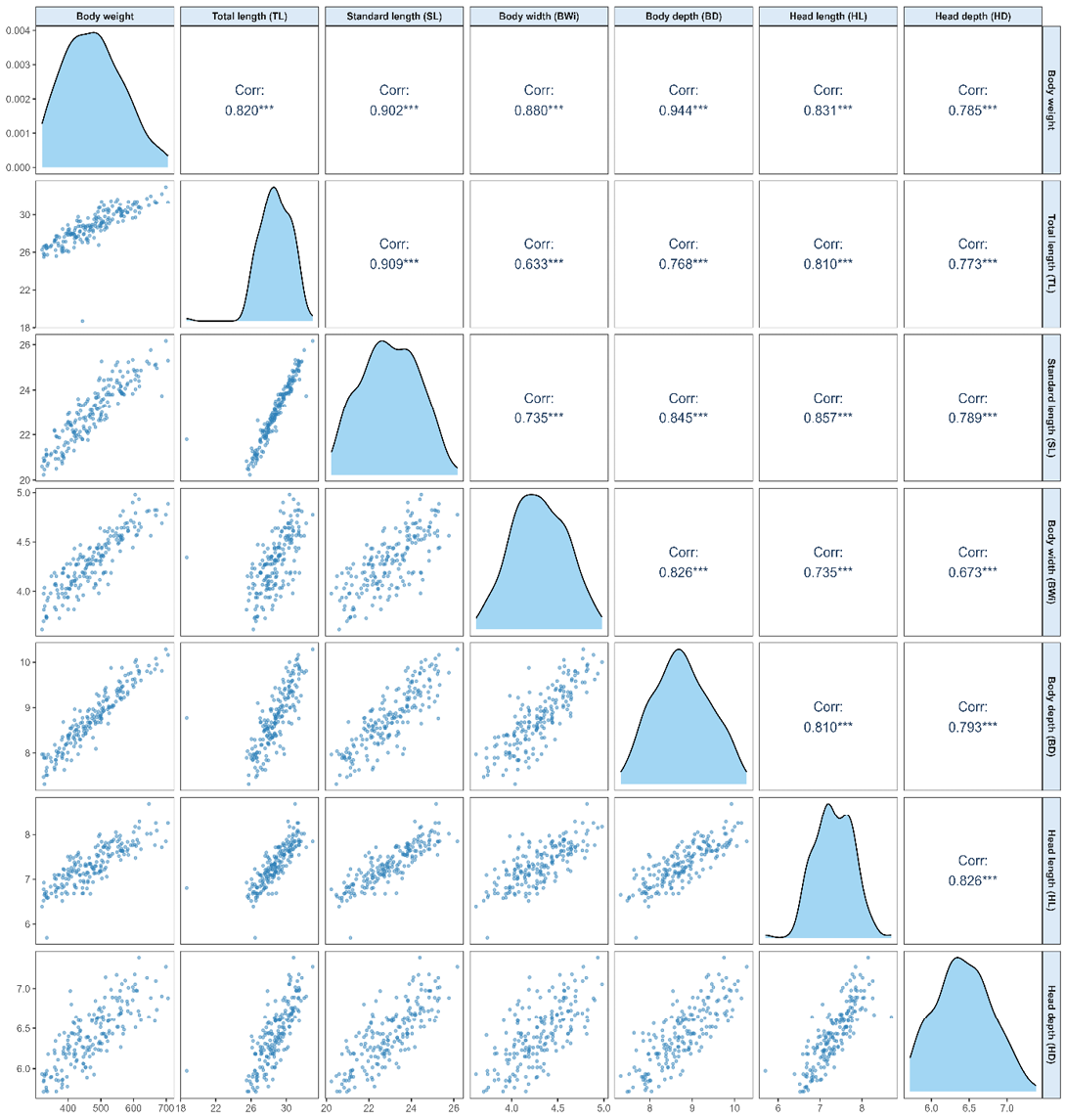
illustrates the Pearson correlation coefficients for the evaluated body traits, including body weight (BW), across the entire dataset. BW showed the strongest positive associations (P < 0.001) with BD, SL, BWi, HL, and TL, with coefficients ranging from 0.82 to 0.94. In addition, a high positive correlation (P < 0.001) was also observed between BW and HD (0.79). Similar findings were reported by Fernandes et al. (2020) and Fernandes et al. (2015) in Nile tilapias, who observed a high correlation between BW and body height (0.96 and 0.94, respectively), which aligns with our result for body depth (0.944). Additionally, these authors reported strong correlations between BW and length measures (0.92 in both studies), though our correlation with total length (0.82) was comparatively lower. Conversely, Azua et al. (2017) reported higher correlations for total length (0.94) and standard length (0.95) with BW, while their correlation for body width (0.27) was substantially lower than our finding (0.88) and those reported by Silva et al. (2018) in the GIFT-Epagri strain (0.900 in males and 0.859 in females). Notably, Silva et al. (2018) also documented strong correlations between BW and head length (0.887 in males and 0.892 in females), which exceeded our value (0.831). The high correlations between BW and BWi found in our study are also in alignment with those reported in other fish species (r= 0.89, Hamzaoui et al., 2023; Firdaus and Supriyadi, 2024). Strong positive correlation (P < 0.001) was observed between SL and TL (0.91). The remaining correlations among body measurements ranged from moderate to high, with values between 0.63 and 0.86.
Table 2: Boruta importance scores for predictors retained after correlation filtering in the final training dataset.
| Traits | meanImp | medianImp | minImp | maxImp | normHits | decision |
| TL | 28.396 | 28.155 | 27.440 | 30.467 | 1.000 | Confirmed |
| BWi | 32.228 | 32.277 | 30.614 | 34.602 | 1.000 | Confirmed |
| HD | 16.459 | 16.410 | 15.121 | 18.016 | 1.000 | Confirmed |
TL: total length; BWi: body width; HD: head depth. SL, BD, and HL were removed during correlation filtering before the final Boruta analysis.
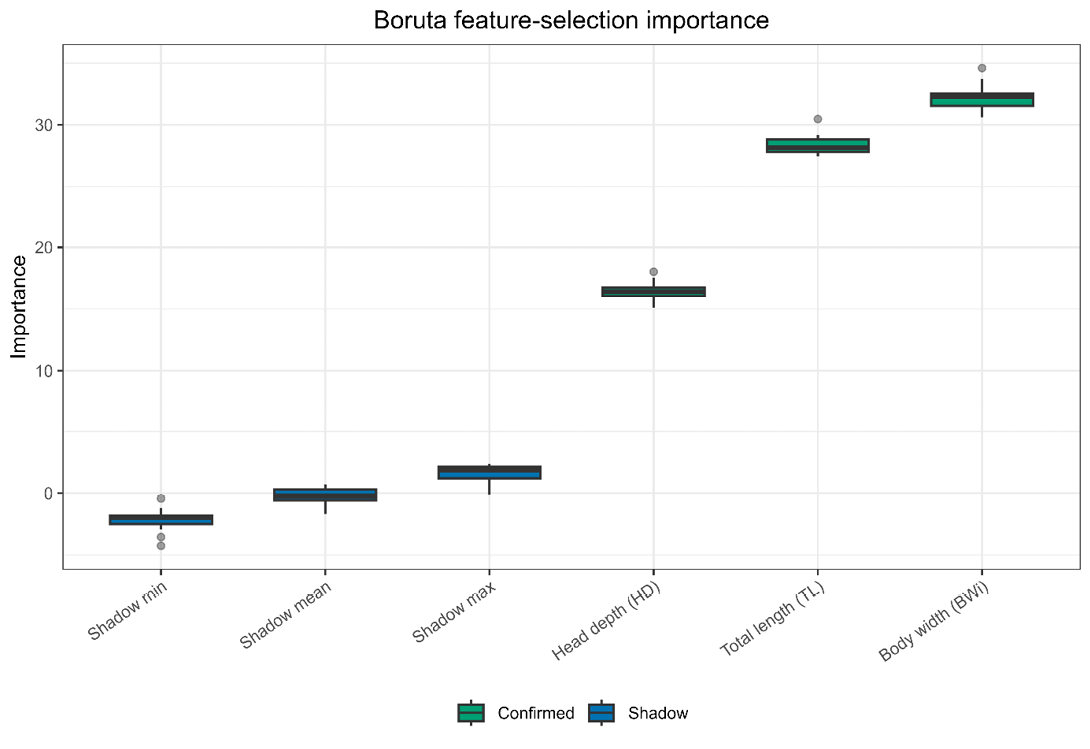
Boruta feature-selection results for predictors retained after correlation filtering in the final training dataset. Green boxplots represent confirmed predictors (TL, BWi, and HD), whereas blue boxplots represent Boruta shadow reference variables. TL: total length; BWi: body width; HD: head depth.
Table 2 and Figure 2 summarize the Boruta feature selection outcomes, confirming BWi (32.23), TL (28.40), and HD (16.46) as relevant predictors of body weight in Nile tilapia, all of them clearly exceeding the maximum shadow importance. Across the 100 outer training folds, BWi and HD were selected in 100% and 99% of resamples, respectively, whereas TL was selected in 62%, and SL, BD, and HL were never retained after correlation filtering (Supplementary Figure S1). Every predictor that passed correlation filtering was subsequently confirmed by Boruta, indicating that the lower selection frequency of TL resulted from correlation filtering, reflecting its high correlation with other length measurements, rather than from Boruta. In addition, Figure 3 depicts the linear associations between body weight and these three predictors, whose correlation coefficients (BWi: 0.88; TL: 0.82; HD: 0.78) followed the same ranking as the Boruta importance scores. To our knowledge, this is the first study to apply Boruta selection in fish morphometric analysis. In other livestock species, the Boruta algorithm has proven useful for identifying the most relevant morphometric predictors of body weight. In sheep, it has highlighted the importance of thoracic measurements, body dimensions, and limb variables ; . Together, these findings suggest that a reduced set of non-redundant measurements can achieve accurate body weight prediction across species.
The predictive performance of the seven models for estimating body weight in Nile tilapia on the independent testing dataset (n= 48) is summarized in Table 3. The ANN, RF, XGBoost, and MARS models achieved the highest and very similar predictive performance, with R² values ranging from 0.920 to 0.923 and RMSE values between 27.40 and 28.10 g. Among them, ANN yielded the lowest error metrics (RMSE: 27.40 g; MAE: 20.94 g; MAPE: 4.40%; CV(RMSE): 5.73%), closely followed by MARS (RMSE: 27.41 g; MAE: 21.03 g; MAPE: 4.40%) and XGBoost (RMSE: 27.70 g; MAE: 21.05 g; MAPE: 4.40%), whereas RF reached the highest R² (0.923) with slightly higher error values (RMSE: 28.10 g; MAE: 21.25 g; MAPE: 4.49%). The SVM model also performed competitively (R²= 0.916; RMSE: 28.45 g; MAE: 22.93 g; MAPE: 4.79%), while CART showed the lowest predictive ability, with an R² of 0.846 and the highest error indicators (RMSE: 38.14 g; MAE: 30.78 g;
Table 3: Predictive performance of the seven models on the independent testing dataset (n = 48).
| Model | R² | RMSE (g) | MAE (g) | MAPE (%) | CV(RMSE) (%) | CV(MAE) (%) |
| ANN | 0.922 | 27.400 | 20.940 | 4.400 | 5.730 | 4.380 |
| CART | 0.846 | 38.140 | 30.780 | 6.540 | 7.980 | 6.440 |
| SVM | 0.916 | 28.450 | 22.930 | 4.790 | 5.950 | 4.800 |
| RF | 0.923 | 28.100 | 21.250 | 4.490 | 5.880 | 4.450 |
| MARS | 0.920 | 27.410 | 21.030 | 4.400 | 5.740 | 4.400 |
| XGBoost | 0.921 | 27.700 | 21.050 | 4.400 | 5.800 | 4.400 |
| MLR | 0.914 | 28.440 | 21.790 | 4.590 | 5.950 | 4.560 |
ANN: artificial neural network; CART: classification and regression tree; SVM: support vector machine with radial basis function kernel; RF: random forest; MARS: multivariate adaptive regression splines; XGBoost: extreme gradient boosting; MLR: multiple linear regression.
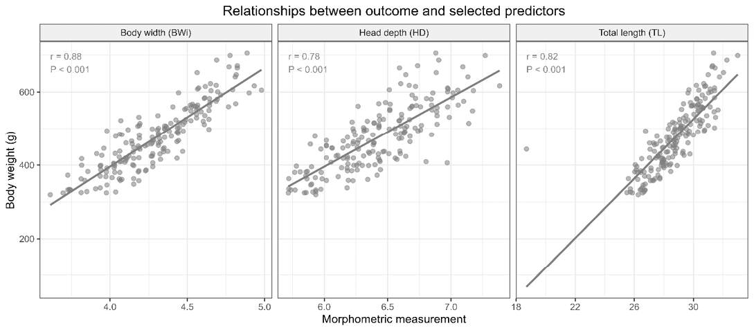
Relationships between body weight and the three final morphometric predictors retained after correlation filtering and Boruta selection. Solid lines represent linear fits; Pearson correlation coefficients (r) and corresponding P-values are shown within each panel. BWi: body width; HD: head depth; TL: total length.
MAPE: 6.54%; CV(RMSE): 7.98%). Notably, the conventional MLR model performed comparably to the ML algorithms (R²= 0.914; RMSE: 28.44 g; MAE: 21.79 g; MAPE: 4.59%), outperforming SVM in terms of MAE and MAPE and differing from the best model by approximately 1 g in RMSE. This suggests that, with the three non-redundant predictors retained, the relationship between morphometric traits and body weight was predominantly linear, so the additional flexibility of the ML algorithms provided only marginal gains in accuracy. These results are broadly consistent with the literature on ML-based body weight prediction in livestock, where ensemble methods such as RF have frequently demonstrated competitive or superior performance ; ; ; . The strong performance of the ML algorithms observed in our study also finds support in reports from other production contexts, including cattle and pigs, where flexible non-linear algorithms have outperformed simpler tree-based models ; ; .
ANN, RF, XGBoost, and MARS models exhibited the highest predictive performance on the testing dataset (Table 3). Figure 4 displays the permutation importance scores, expressed as the increase in MAE (g), of the three final predictors for each model. Across all seven models, including MLR, BWi and TL were consistently identified as the most influential predictors of body weight, with BWi ranking first in ANN, CART, RF, XGBoost, and MLR (29.51–39.39 g), and TL ranking first in SVM and MARS (37.93 and 34.93 g, respectively). In contrast, HD made only a marginal contribution in most models (0.77–7.02 g), with its lowest importance observed in MARS (0.77 g); SVM was the only model in which HD showed a moderate contribution (13.14 g). The dominant role of BWi and TL as predictors of body weight in Nile tilapia is consistent with prior research demonstrating the
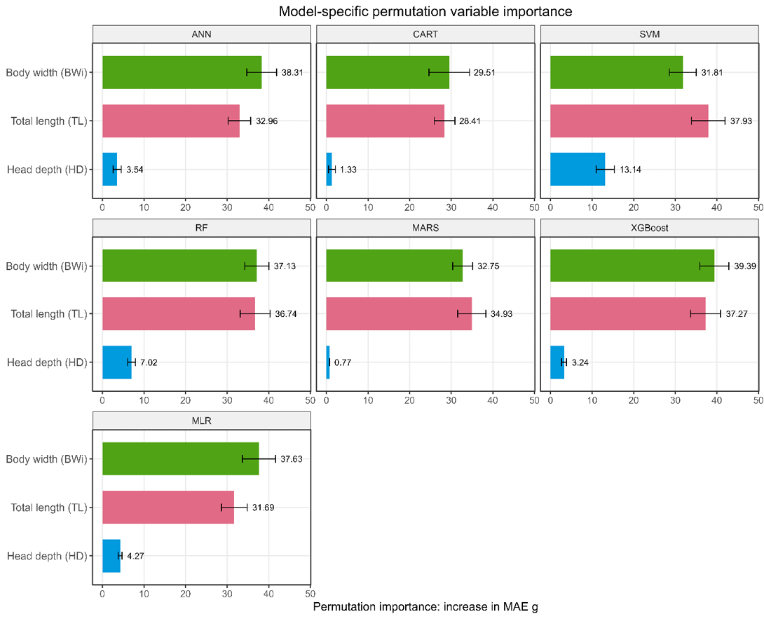
Model-specific permutation importance of the three final predictors for ANN, CART, SVM, RF, MARS, XGBoost, and MLR. Importance was quantified as the increase in MAE (g) after predictor permutation. Error bars represent variability across repeated permutations. BWi: body width; TL: total length; HD: head depth.
strong biological association between body measurements and body mass in fish . Tengtrairat et al. (2022) employed deep learning for object detection combined with classical regression models to estimate the weight of farmed tilapia. They concluded that these approaches require only age and three morphometric dimensions (length, width, and depth) to estimate the fish’s weight. To the best of the authors’ knowledge, no previous study has simultaneously compared the algorithms used in this study for predicting body weight of Nile tilapia from manually measured morphometric traits. In other livestock species, longitudinal and thoracic body measurements have consistently emerged as dominant predictors of body weight across ML models. In Corriedale sheep, wither height, thoracic perimeter, fore-shank length, loin width, shoulder width, and body length were identified as primary variables by RF and XGBoost , while chest circumference, chest depth, and shoulder width were the dominant predictors in RF for Suffolk and Polish Merino crossbred sheep . In Balochi sheep, body length alone accounted for approximately 35% of the variation in body weight under the RF model . Similarly, Faraz et al. (2023) reported that body length, height at withers, and rump width were the most reliable predictors for Kajli sheep using XGBoost. Collectively, these findings suggest that a reduced set of key body measurements tends to drive predictive accuracy in ML-based models, a pattern consistent with the dominant role of BWi and TL observed in the present study.
Table 4 presents the mean, standard deviation (SD), and 95% interval of the performance metrics across 100 outer validation resamples of repeated nested cross-validation. Under this more rigorous assessment, MLR achieved the best mean performance (R²= 0.889; RMSE= 28.64 g;
Table 4: Predictive performance across 100 outer validation resamples of repeated nested cross-validation.
| Model | Criterion | Mean | SD | Lower 95% | Upper 95% |
| ANN | RMSE (g) | 29.370 | 9.490 | 16.340 | 51.740 |
| MAE (g) | 23.110 | 7.880 | 12.890 | 41.220 | |
| R² | 0.883 | 0.085 | 0.646 | 0.966 | |
| CART | RMSE (g) | 37.550 | 8.980 | 20.990 | 56.950 |
| MAE (g) | 30.270 | 7.570 | 16.040 | 46.510 | |
| R² | 0.822 | 0.080 | 0.657 | 0.935 | |
| SVM | RMSE (g) | 34.080 | 11.320 | 19.100 | 56.200 |
| MAE (g) | 26.650 | 8.220 | 15.050 | 44.250 | |
| R² | 0.851 | 0.095 | 0.629 | 0.958 | |
| RF | RMSE (g) | 30.900 | 9.020 | 16.960 | 51.740 |
| MAE (g) | 24.630 | 7.520 | 13.610 | 42.730 | |
| R² | 0.875 | 0.079 | 0.689 | 0.967 | |
| MARS | RMSE (g) | 29.270 | 9.310 | 17.020 | 50.670 |
| MAE (g) | 22.930 | 7.740 | 12.960 | 41.590 | |
| R² | 0.886 | 0.075 | 0.695 | 0.967 | |
| XGBoost | RMSE (g) | 32.720 | 10.090 | 17.830 | 56.680 |
| MAE (g) | 25.650 | 8.270 | 14.050 | 47.170 | |
| R² | 0.860 | 0.092 | 0.618 | 0.955 | |
| MLR | RMSE (g) | 28.640 | 9.520 | 16.060 | 50.730 |
| MAE (g) | 22.330 | 7.660 | 13.030 | 42.390 | |
| R² | 0.889 | 0.079 | 0.683 | 0.971 |
ANN: artificial neural network; CART: classification and regression tree; SVM: support vector machine with radial basis function kernel; RF: random forest; MARS: multivariate adaptive regression splines; XGBoost: extreme gradient boosting; MLR: multiple linear regression.
MAE= 22.33 g), closely followed by MARS (R²= 0.886; RMSE= 29.27 g; MAE= 22.93 g) and ANN (R²= 0.883; RMSE= 29.37 g; MAE= 23.11 g), whereas RF (R²= 0.875), XGBoost (R²= 0.860), and SVM (R²= 0.851) showed intermediate performance, and CART again yielded the lowest predictive ability (R² = 0.822; RMSE= 37.55 g; MAE= 30.27 g). The differences among the best-performing models were small relative to the variability across resamples, as reflected in the wide and largely overlapping 95% intervals (e.g., R² ranging approximately from 0.62 to 0.97), indicating that performance estimates were sensitive to the composition of the validation folds. SVM showed the greatest variability in RMSE (SD= 11.32 g), followed by XGBoost (SD = 10.09 g), whereas MARS showed the lowest SD for R² (0.075). These results are consistent with those obtained on the independent testing dataset, where MLR performed comparably to the ML algorithms, and reinforce that, with the three non-redundant predictors retained, the relationship between morphometric traits and body weight was largely linear. This contrasts with previous studies in fish species, where RF and XGBoost outperformed linear and simpler tree-based models such as Decision Tree for body weight estimation ; ; , although the advantage of ensemble methods over CART reported in those studies was also evident here. The Friedman test indicated significant differences among models in fold-level RMSE (χ² = 193.80, df = 6, P < 0.001) and MAE (χ² = 219.84, df = 6, P < 0.001). Pairwise Wilcoxon signed-rank tests with Holm correction (Supplementary Figure S2) showed no significant differences between MLR and MARS (RMSE: P = 0.191; MAE: P= 0.062) or between MARS and ANN (RMSE: P = 0.480; MAE: P= 0.438), whereas MLR showed slightly but significantly lower errors than ANN (RMSE: P = 0.029; MAE: P= 0.003). These three models had significantly lower errors than RF, XGBoost, SVM, and CART; RF outperformed XGBoost and SVM, which did not differ from each other (RMSE: P= 0.352; MAE: P= 0.059), and CART showed significantly higher errors than all other models (P < 0.001). However, the median paired differences among MLR, MARS, and ANN were below 1 g in RMSE, indicating limited practical relevance. Because outer resamples share training observations, these P-values should be interpreted as supporting evidence rather than as strictly independent tests. The learning curves for all models, generated using the training dataset only, are presented in Figure 5. As the training subset size increased, validation errors generally decreased and then stabilized, whereas training errors tended to increase slightly, leading to a narrowing of the gap between training and validation performance in most models. MLR, MARS, and ANN showed the closest agreement between training and validation curves at the full training subset size, with R² values converging at approximately 0.87–0.88, indicating good generalization without marked overfitting. In contrast, RF maintained consistently low training errors (RMSE ≈ 15 g) and a relatively flat validation curve (RMSE ≈ 33–37 g) across all subset sizes, resulting in the widest and most persistent gap between training and validation performance, which reflects the tendency of this ensemble method to closely fit the training data. XGBoost exhibited a similar pattern, with very low and irregular training errors at small subset sizes and a gradual reduction in validation error. SVM and CART showed the highest validation errors at the smallest training subset size (RMSE ≈ 50 g), followed by a sharp decrease and subsequent stabilization, although CART retained the highest error levels throughout. MARS and MLR displayed non-monotonic fluctuations in validation error at intermediate subset sizes, but these were of limited magnitude and both models converged to stable values. The close convergence of MLR, MARS, and ANN, contrasted with the persistent training–validation gaps of RF, XGBoost, SVM, and CART, is consistent with findings in other animal species highlighting the differential sensitivity of these algorithms to training data size , 2025). Similarly, MARS and XGBoost have demonstrated strong predictive performance for body weight estimation from morphometric traits in other animal production contexts , further supporting the applicability of these algorithms beyond fish species.
To further evaluate the agreement between observed and predicted values, a Bland–Altman analysis was performed (Figure 7). All models showed a mean prediction bias close to zero (−2.86 to +4.46 g), indicating no relevant systematic over- or underestimation of body weight. The 95% limits of agreement were similar for ANN, SVM, RF, MARS, XGBoost, and MLR (ranging from −58.59 to +57.29 g), whereas CART showed the widest limits (−70.58 to +79.49 g), consistent with its lower predictive accuracy (Table 3). Most observations fell within the limits of agreement for all models. The regression of prediction differences on the mean of observed and predicted values yielded negative slopes for all models, confirming the tendency to underestimate the heaviest
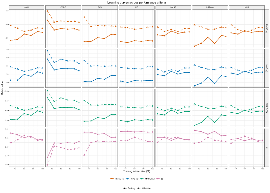
Learning curves for the seven prediction models across increasing training-subset sizes. Rows represent RMSE, MAE, MAPE, and R². Solid lines with circles represent training performance, whereas dashed lines with triangles represent validation performance. Learning curves were generated using the training dataset only; the independent testing dataset was not used.
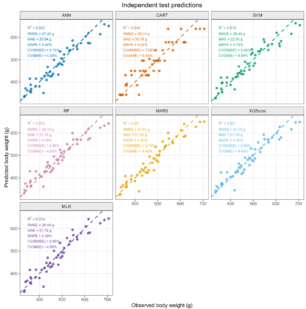
displays the relationship between observed and predicted body weight for the seven models on the independent testing dataset (n= 48), together with the goodness-of-fit metrics reported in Table 3. For all models except CART, predictions were closely distributed around the 1:1 line, with R² values ranging from 0.914 (MLR) to 0.923 (RF). CART showed the greatest dispersion (R² = 0.846) and a stepwise prediction pattern, in which fish with different observed weights received identical predicted values, reflecting the limited number of terminal nodes of a single regression tree. In all models, the heaviest fish (observed body weight above approximately 600 g) tended to fall below the 1:1 line, indicating underestimation at the upper end of the weight range. In addition, one individual with an observed body weight of approximately 420 g was consistently underestimated by all models (predicted ≈ 345 g).
fish identified in Figure 6; however, this proportional bias was statistically significant only for RF (P = 0.002), SVM (P = 0.019), and XGBoost (P = 0.021), and borderline for ANN (P= 0.051). This trend likely reflects the smaller number of large individuals in the dataset. In addition, the individual underestimated by all models appeared among the largest negative differences, suggesting an atypical observation rather than a model-specific error. Overall, the Bland–Altman analysis showed that, apart from CART, the models exhibited comparable agreement with observed body weight, in line with the small differences observed in the goodness-of-fit metrics. Computational requirements differed markedly among models (Supplementary Table S2).
Training and hyperparameter tuning on the complete training dataset required less than 0.01 s for MLR, between 0.83 and 5.03 s for CART, SVM, MARS, and RF, 27.11 s for ANN, and 121.11 s for XGBoost, whereas prediction time was below 0.11 ms per observation for all models. Therefore, although training costs differed by more than two orders of magnitude, inference time was negligible for all models and would not constrain practical on-farm use.
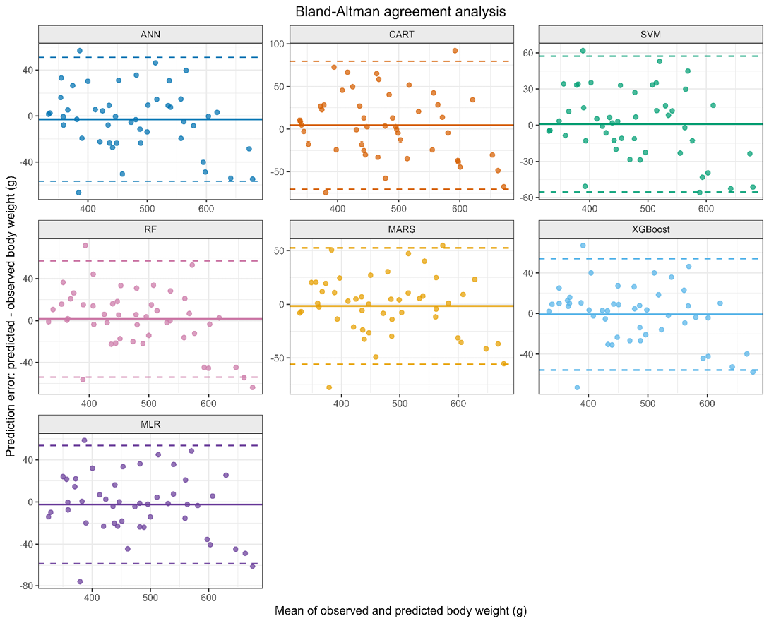
Bland–Altman agreement analysis between observed and predicted body weight on the independent testing dataset (n = 48). The solid horizontal line represents the mean prediction bias (predicted − observed body weight), and the dashed lines represent the 95% limits of agreement (mean bias ± 1.96 SD of the prediction differences).
Overall, body weight in Nile tilapia could be estimated with good accuracy from a small set of morphometric traits, with all models except CART showing comparable performance. No single algorithm consistently outperformed the others: MLR achieved the best mean performance under repeated nested cross-validation, closely followed by MARS, whereas ANN yielded the lowest errors and RF the highest R² on the independent testing dataset. Thus, consistency across validation strategies is more meaningful than the superiority of any individual algorithm. The competitive performance of MLR and the near-zero bias in the Bland–Altman analysis suggest a largely linear relationship between the retained predictors and body weight, supporting the continued usefulness of linear models for weight prediction from morphometric data ; , 2021; . Biologically, the predominant contribution of BWi and TL reflects their joint representation of body volume ; , whereas HD, which reflects cranial size, was consistently selected (99% of resamples) but contributed little additional information beyond BWi and TL. However, the dataset comprises a relatively small sample (n= 185) from a single population with a limited weight range, which limits the precision of comparisons among models, particularly for data-intensive algorithms such as ANN and XGBoost, and all models tended to underestimate the heaviest fish; therefore, the present results represent internal validation in clinically healthy fish reared in a single recirculation system, and external validation across strains, age groups, farms, production systems, environmental conditions, and health states is required. Moreover, because morphometric measurement still requires fish handling, this approach should be regarded as a low-cost alternative to direct weighing rather than a fully non-invasive method, and automated image-based measurement could improve its scalability ; .
Conclusions
Under the conditions studied, body weight in Nile tilapia was predicted with promising accuracy from a reduced set of morphometric traits, with BWi and TL as the main contributors and HD providing only marginal, model-dependent information. Except for CART, all seven models evaluated, including the conventional MLR, showed comparable predictive performance, and no single algorithm consistently outperformed the others across repeated nested cross-validation and the independent testing dataset. The competitive performance of MLR indicates that, with these predictors, a simple and interpretable linear model may be sufficient, whereas more complex ML algorithms provided only marginal gains. Mean prediction bias was close to zero for all models, although the body weight of the heaviest fish tended to be underestimated. These results support morphometric-based prediction as a practical, low-cost alternative to direct weighing in Nile tilapia; however, because it still requires fish handling, it should not be regarded as fully non-invasive, and it should be validated in other populations, weight ranges, and production systems before broader application.
Acknowledgements
The authors gratefully acknowledge the financial support provided by FAPEMIG (Fundação de Amparo à Pesquisa do Estado de Minas Gerais, process number 5.02/2022), CAPES (Coordenação de Aperfeiçoamento de Pessoal de Nível Superior), and CNPq (Conselho Nacional de Desenvolvimento Científico e Tecnológico), as well as the Federal University of Lavras, Brazil, for providing the infrastructure and resources necessary for the development of this study.
Novelty Statement
To the best of our knowledge, this is the first study to simultaneously compare six machine learning algorithms with multiple linear regression for predicting body weight of Nile tilapia from manually measured morphometric traits. A leakage-controlled repeated nested cross-validation strategy was used, together with an independent testing dataset for final evaluation and the Boruta feature-selection method. The results show that body width and total length are the main predictors of body weight.
Author’s Contribution
RC-H: Methodology, formal analysis, investigation, writing original draft. DCO: Methodology, investigation, writing review and editing. AWC-C: Methodology, investigation, writing review and editing, formal analysis. ALM: Formal analysis, investigation, writing original draft. MG, CÇ and RB: Methodology. RTFF: Resources, funding acquisition, writing review and editing.
Data availability
The data presented in this study are available upon reasonable request from the corresponding author.
Code availability
The R script used for the analyses will be made available by the corresponding author upon reasonable request after acceptance of the article.
Ethics approval
Not applicable.
Consent for publication
All the authors consent to publish the manuscript.
Generative AI and AI assisted technology statement
During the preparation of this manuscript, the authors used Claude (Anthropic) exclusively for language refinement, including grammar checking and improvements in clarity and readability. The authors independently developed and verified all scientific content and take full responsibility for the final manuscript
Conflict of interest
The authors have declared no conflict of interest.
References
- Azis R, Ciptadi G, Wahjuningsih S, Hariyono DNH, Tribudi YA, Nurgiartiningsih VMA (2023). Prediction of body weight from body measurements in Bali cattle of Indonesia using regression analysis. Adv. Anim. Vet. Sci., 11(9): 1486–1491. https://doi.org/10.17582/journal.aavs/2023/11.9.1486.1491 [CrossRef]
- Azua ET, Akaahan TJ, Akogwu SA (2017). Variation in the morphometry measurements of two tilapia fish species in relation to their body weight obtained from Lower Benue River at Makurdi, Benue State Nigeria. Fish Aquacult. J., 8(208): 2. [CrossRef]
- Bland JM, Altman DG (1986). Statistical methods for assessing agreement between two methods of clinical measurement. Lancet, 327(8476): 307–310. https://doi.org/10.1016/S0140-6736(86)90837-8 [CrossRef]
- Çakmakçı C (2022). Live weight prediction in Norduz sheep using machine learning algorithms. Turk. J. Agricult. Food Sci. Technol., 10(4): 587–594. https://doi.org/10.24925/turjaf.v10i4.587-594.4670 [CrossRef]
- Canaza-Cayo AW, Beltrán Barriga PA, Gallegos Rojas E, Mayta-Quispe J (2017). Zoometría y estimación de ecuaciones de predicción de peso vivo en ovejas de la raza Corriedale. Rev. Invest. Altoand., 19(3): 313–318. https://doi.org/10.18271/ria.2017.296 [CrossRef]
- Canaza-Cayo AW, Churata-Huacani R, Çakmakçı C, Rodríguez-Huanca FH, de Sousa BFJS, Fernandes TJ, Rojas YC (2024). Use of machine learning approaches for body weight prediction in Peruvian Corriedale sheep. Smart Agric. Technol., 7: 100419. https://doi.org/10.1016/j.atech.2024.100419 [CrossRef]
- Canaza-Cayo AW, Mota RR, Amarilho-Silveira F, Duarte DAS, Cobuci JA (2021). Principal component analysis for body weight prediction of Corriedale ewes from southern Peru. J. Anim. Health Prod., 9(4): 417–424. https://doi.org/10.17582/journal.jahp/2021/9.4.417.424 [CrossRef]
- Canaza-Cayo AW, Rodríguez-Huanca FH, Huanca-Ilaquijo MC, Carvalheiro R, Romero-Torres MT, Yucra-Yucra YB, Churata-Huacani R (2025). Machine learning algorithm approaches for predicting body weight in tuis Huacaya alpacas. Smart Agric. Technol., 12: 101565. https://doi.org/10.1016/j.atech.2025.101565 [CrossRef]
- Chan E (2023). Prediction of beef cattle body weight based on morphometric measurements extracted from 2D images (Master of Science dissertation, University of Guelph). https://atrium.lib.uoguelph.ca/items/b509be10-0b2a-4d38-9a86-b8d80e411e09
- Dakhlan A, Saputra A, Hamdani MDI, Sulastri (2020). Regression models and correlation analysis for predicting body weight of female Ettawa Grade goat using its body measurements. Adv. Anim. Vet. Sci., 8(11): 1142–1146. https://doi.org/10.17582/journal.aavs/2020/8.11.1142.1146 [CrossRef]
- Faraz A, Tırınk C, Önder H, Şen U, Ishaq HM, Tauqir NA, Waheed A, Nabeel MS (2023). Usage of the XGBoost and MARS algorithms for predicting body weight in Kajli sheep breed. Trop. Anim. Health Prod., 55(4): 276. https://doi.org/10.1007/s11250-023-03700-6 [CrossRef]
- Fernandes AFA, Silva M de A, Alvarenga ER de, Teixeira E de A, Silva Junior AF da, Alves GFde O, Salles SCM de, Manduca LG, Turra EM (2015). Morphometric traits as selection criteria for carcass yield and body weight in Nile tilapia (Oreochromis niloticus L.) at five ages. Aquaculture, 446: 303–309. https://doi.org/10.1016/j.aquaculture.2015.05.009 [CrossRef]
- Fernandes AFA, Turra EM, de Alvarenga ÉR, Passafaro TL, Lopes FB, Alves GFO, Singh V, Rosa GJM (2020). Deep Learning image segmentation for extraction of fish body measurements and prediction of body weight and carcass traits in Nile tilapia. Comput. Electron. Agric., 170: 105274. https://doi.org/10.1016/j.compag.2020.105274 [CrossRef]
- Firdaus N, Supriyadi A (2024). A comparative study on artificial neural networks and random forests for fish weight prediction. Proceedings 2024 17th International Congress on Advanced Applied Informatics, IIAI-AAI-Winter 2024, pp. 25–30. https://doi.org/10.1109/IIAI-AAI-Winter65925.2024.00014 [CrossRef]
- Gilbert RC, Richman MB, Trafalis TB, Leslie LM (2010). Machine learning methods for data assimilation. In Computational intelligence in architecturing complex engineering systems. ASME Press. pp. 105–112. https://doi.org/10.1115/1.859599.paper14 [CrossRef]
- Hamzaoui M, Aoueileyine MOE, Romdhani L, Bouallegue R (2023). Optimizing XGBoost performance for fish weight prediction through parameter pre-selection. Fishes, 8(10): 505. https://doi.org/10.3390/fishes8100505 [CrossRef]
- Hassan N, Kadir STSA, Husain ML, Satyanarayana B, Ambak MA, Ghaffar AM (2023). Weight prediction for fishes in Setiu wetland, Terengganu, using machine learning regression model. BIO Web of Conferences, 73: 01007. https://doi.org/10.1051/bioconf/20237301007 [CrossRef]
- Huma ZE, Iqbal F (2019). Predicting the body weight of Balochi sheep using a machine learning approach. Turk. J. Vet. Anim. Sci., 43(4): 500–506. https://doi.org/10.3906/vet-1812-23 [CrossRef]
- Khalid M, Naeem M, Azam SM, Ahmad N, Kausar S, Mustafa G, Asad M, Qureshi H, Atiq I, Raza S, Faiz M, Khakwani AZ, Irshad S, Riaz P, Lal V, Rehman NU, Khursheed Z (2023). Morphometric and length-weight relationship of the Nile tilapia (Oreochromis niloticus (Linnaeus, 1758) from Head Panjnad, Punjab, Pakistan. Egypt. J. Aquat. Biol. Fish., 27(2): 25–33. https://doi.org/10.21608/ejabf.2023.289096 [CrossRef]
- Kuhn M (2025). Caret: Classification and regression training (R package version 7.0-1). https://CRAN.R-project.org/package=caret
- Kunene NW, Nesamvuni AE, Nsahlai IV (2009). Determination of prediction equations for estimating body weight of Zulu (Nguni) sheep. Small Rumin. Res., 84(1–3): 41–46. https://doi.org/10.1016/j.smallrumres.2009.05.003 [CrossRef]
- Kursa MB, Rudnicki WR (2010). Feature selection with the boruta package. J. Statist. Software, 36(11): 1–13. https://doi.org/10.18637/jss.v036.i11 [CrossRef]
- PeixeBR, Associação Brasileira de Piscicultura (2018). Anuário PeixeBR da piscicultura 2018. https://www.peixebr.com.br/anuario2018
- Portillo-Salgado R, Sánchez-Márquez AY, Oney-Montalvo JE, Dzib Cauich DA, de Jesús Chi-Gutiérrez E (2025). Relationship between body weight, body measurements and carcass characteristics of Nile tilapia (Oreochromis niloticus L.). Biotechnol. Anim. Husband., 41(1): 25-35. https://doi.org/10.2298/BAH2501025P [CrossRef]
- R Core Team (2025). R: A language and environment for statistical computing. R foundation for statistical computing. https://www.R-project.org/
- Rotondo V, Tulpan D, Wood KM, Paibomesai M, Osborne VR (2021). PSIII-5 Predicting live weight using linear body measurements in growing beef calves. J. Anim. Sci., 99(Supplement_3): 285–285. https://doi.org/10.1093/jas/skab235.523 [CrossRef]
- Sant’Ana DA, Pache MCB, Martins J, Soares WP, de Melo SLN, Garcia V, de Moares Weber VA, da Silva Heimbach N, Mateus RG, Pistori H (2021). Weighing live sheep using computer vision techniques and regression machine learning. Machine Learn. Appl., 5: 100076. https://doi.org/10.1016/j.mlwa.2021.100076 [CrossRef]
- Silva BC, Marchiori NC, Silva FM (2018). Morphometric measurements and phenotypic correlations of the tilapia Gift after individual selection (2018). Agropecuária Catarinense, 31(3): 38–40. https://doi.org/10.22491/RAC.2018.v31n3.3 [CrossRef]
- Tengtrairat N, Woo WL, Parathai P, Rinchumphu D, Chaichana C (2022). Non-intrusive fish weight estimation in turbid water using deep learning and regression models. Sensors, 22(14): 5161. https://doi.org/10.3390/s22145161 [CrossRef]
- Tırınk C, Piwczyński D, Kolenda M, Önder H (2023). Estimation of body weight based on biometric measurements by using random forest regression, support vector regression and CART Algorithms. Animals, 13(5): 798. https://doi.org/10.3390/ani13050798 [CrossRef]
- Wang Z (2023). Comparison of machine learning algorithms for estimation of pig body weights from on-animal and digital image measurements. Master of Science dissertation, University of Guelph.
- Ye X, Abe S, Zhang S (2020). Estimation and mapping of nitrogen content in apple trees at leaf and canopy levels using hyperspectral imaging. Precision Agric., 21(1): 198–225. https://doi.org/10.1007/s11119-019-09661-x [CrossRef]
Supplementary material

Services
Article usage statistics
Loading…
Related articles
- Comparing the Predictive Ability of Machine Learning Methods in Predicting the Live Body Weight of Beetal Goats of PakistanPakistan Journal of Zoology · 2021
- Comparative Study of Growth, Hematology and Proximate Composition of Nile Tilapia (Oreochromis niloticus) in Biofloc Technology and Conventional Pond Culture SystemPakistan Journal of Zoology · 2025
- Comparing Predictive Performances of Tree-Based Data Mining Algorithms and MARS Algorithm in the Prediction of Live Body Weight from Body Traits in Pakistan GoatsPakistan Journal of Zoology · 2019
- Effect of Allium sativum Supplemented Diets on Growth and Haematological Responses in Nile Tilapia (Oreochromis niloticus)Pakistan Journal of Zoology · 2018
- Prediction of Live Body Weight for Thalli Sheep Using Chi-Square Automatic Interaction Detector and Multiple Linear Regression: A Comparative StudyPakistan Journal of Zoology · 2022
- Assessment of Optimum Salinity Level for Maximum Growth and Survival of Nile Tilapia, Oreochromis niloticus (Linnaeus 1758)Pakistan Journal of Zoology · 2018